seaborn.heatmap

Heat maps display numeric tabular data where the cells are colored depending upon the contained value. Heat maps are great for making trends in this kind of data more readily apparent, particularly when the data is ordered and there is clustering.

dataset: Seaborn - flights

%matplotlib inline
import pandas as pd
import matplotlib.pyplot as plt
import seaborn as sns
import numpy as np
plt.rcParams['figure.figsize'] = (20.0, 10.0)
plt.rcParams['font.family'] = "serif"

df = pd.pivot_table(data=sns.load_dataset("flights"),
                    index='month',
                    values='passengers',
                    columns='year')
df.head()

year	1949	1950	1951	1952	1953	1954	1955	1956	1957	1958	1959	1960
month
January	112	115	145	171	196	204	242	284	315	340	360	417
February	118	126	150	180	196	188	233	277	301	318	342	391
March	132	141	178	193	236	235	267	317	356	362	406	419
April	129	135	163	181	235	227	269	313	348	348	396	461
May	121	125	172	183	229	234	270	318	355	363	420	472

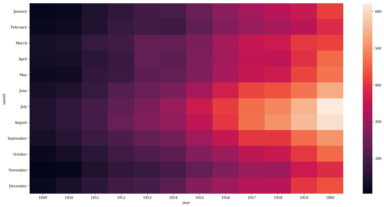
Default plot

sns.heatmap(df)

<matplotlib.axes._subplots.AxesSubplot at 0x10c53b7b8>

png

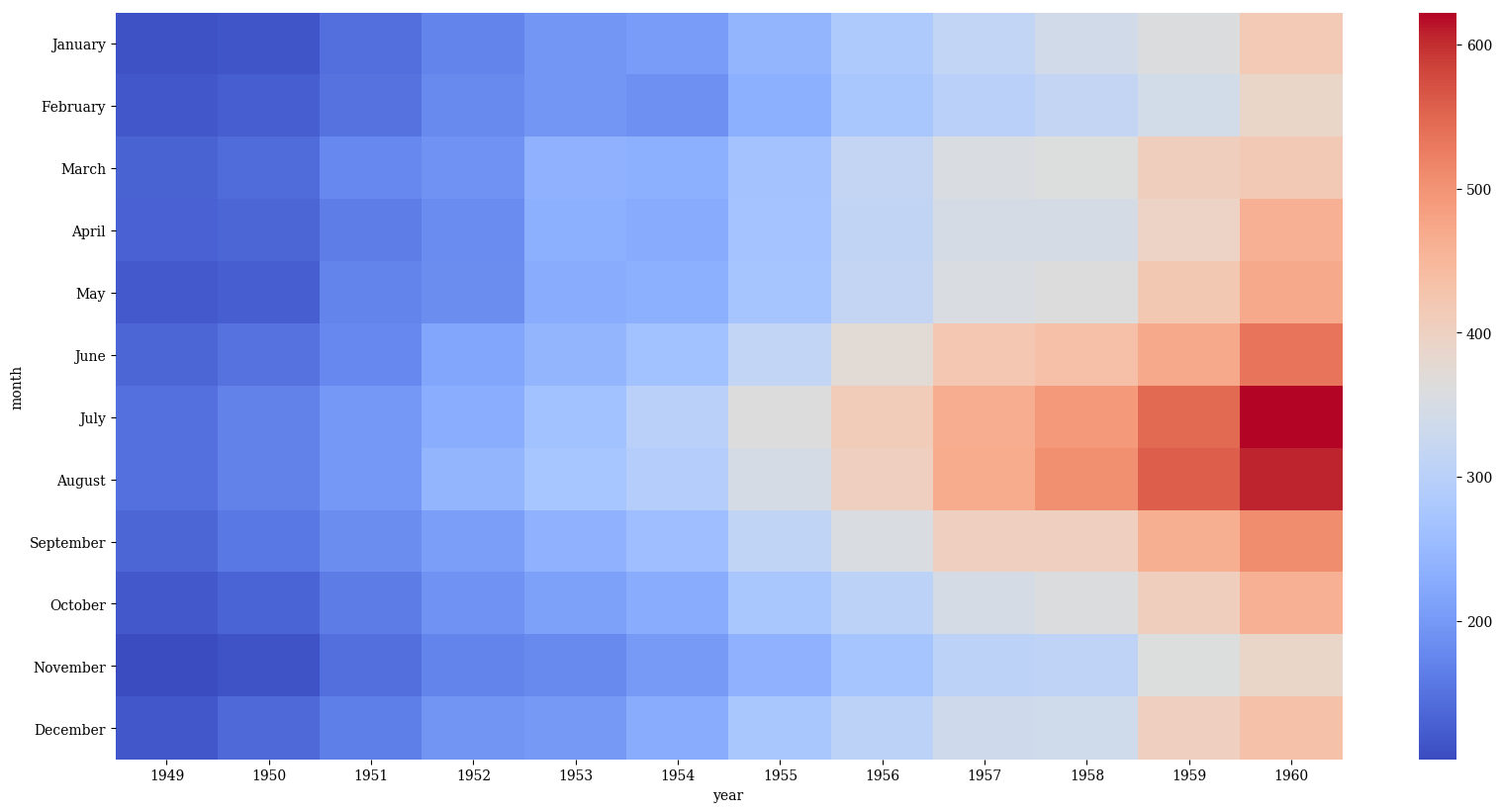
cmap adjusts the colormap used. I like diverging colormaps for heatmaps because they provide good contrast.

sns.heatmap(df, cmap='coolwarm')

<matplotlib.axes._subplots.AxesSubplot at 0x10c65d710>

png

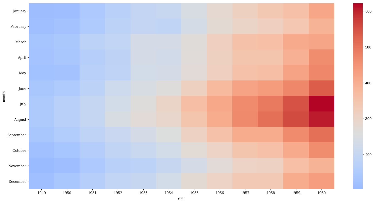
center can be used to indicate at which numeric value to use the center of the colormap. Above we see most of the map using blues, so by setting the value of center equal to the midpoint of the data then we can create a map where there are more equal amounts of red and blue shades.

midpoint = (df.values.max() - df.values.min()) / 2
sns.heatmap(df, cmap='coolwarm', center=midpoint)

<matplotlib.axes._subplots.AxesSubplot at 0x10d448860>

png

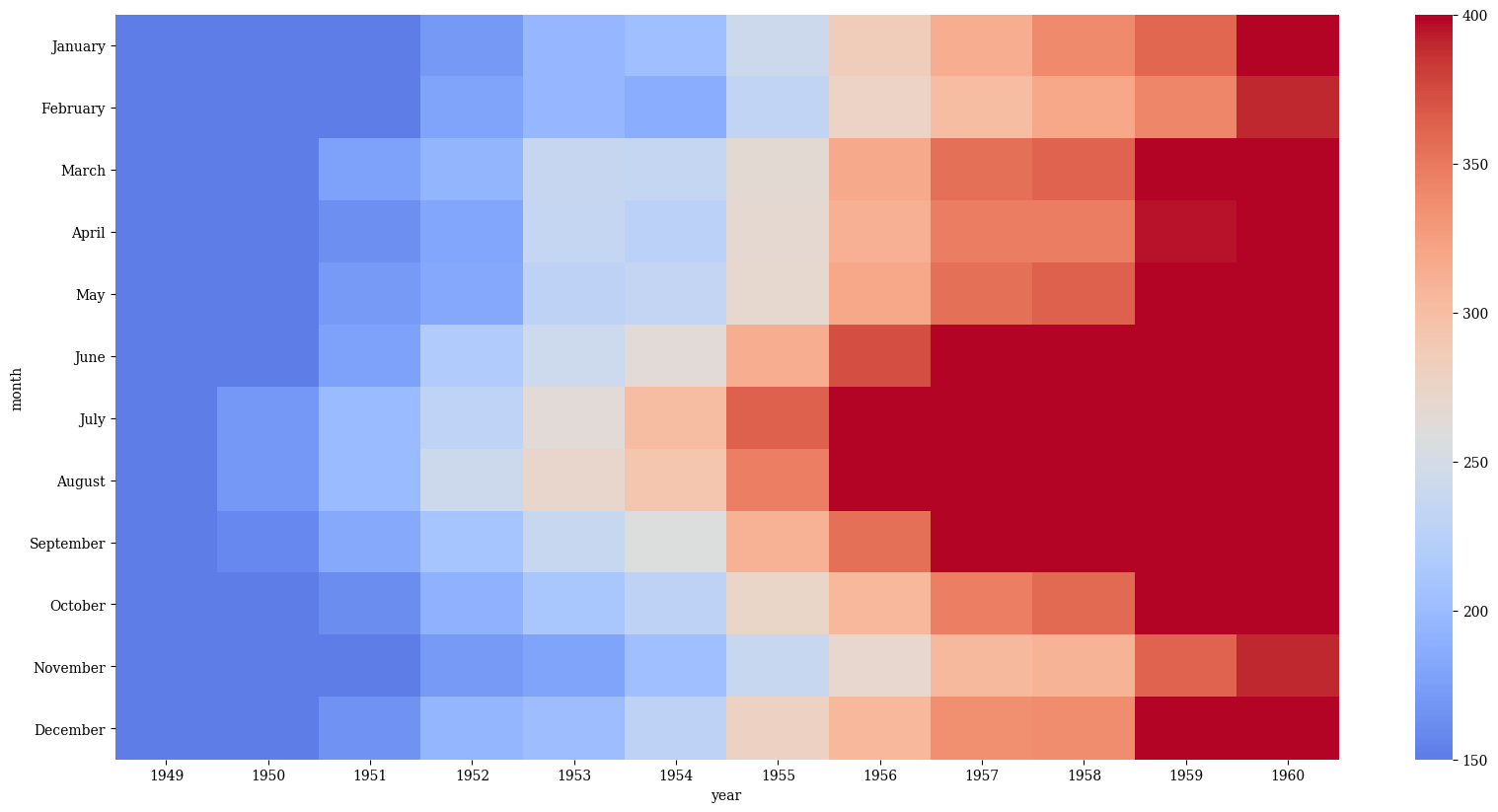
Adjust the lower and upper contrast bounds with vmin and vmax. Everything below vmin will be the same color. Likewise for above vmax.

midpoint = (df.values.max() - df.values.min()) / 2
sns.heatmap(df, cmap='coolwarm', center=midpoint, vmin=150, vmax=400)

<matplotlib.axes._subplots.AxesSubplot at 0x10da59a90>

png

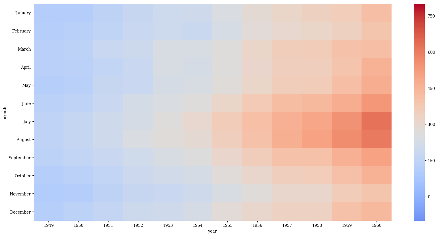
Alternatively, you can set vmin and vmax to lie outside of the range of the data for a more muted, washed-out look

midpoint = (df.values.max() - df.values.min()) / 2
sns.heatmap(df, cmap='coolwarm', center=midpoint, vmin=-100, vmax=800)

<matplotlib.axes._subplots.AxesSubplot at 0x10e038470>

png

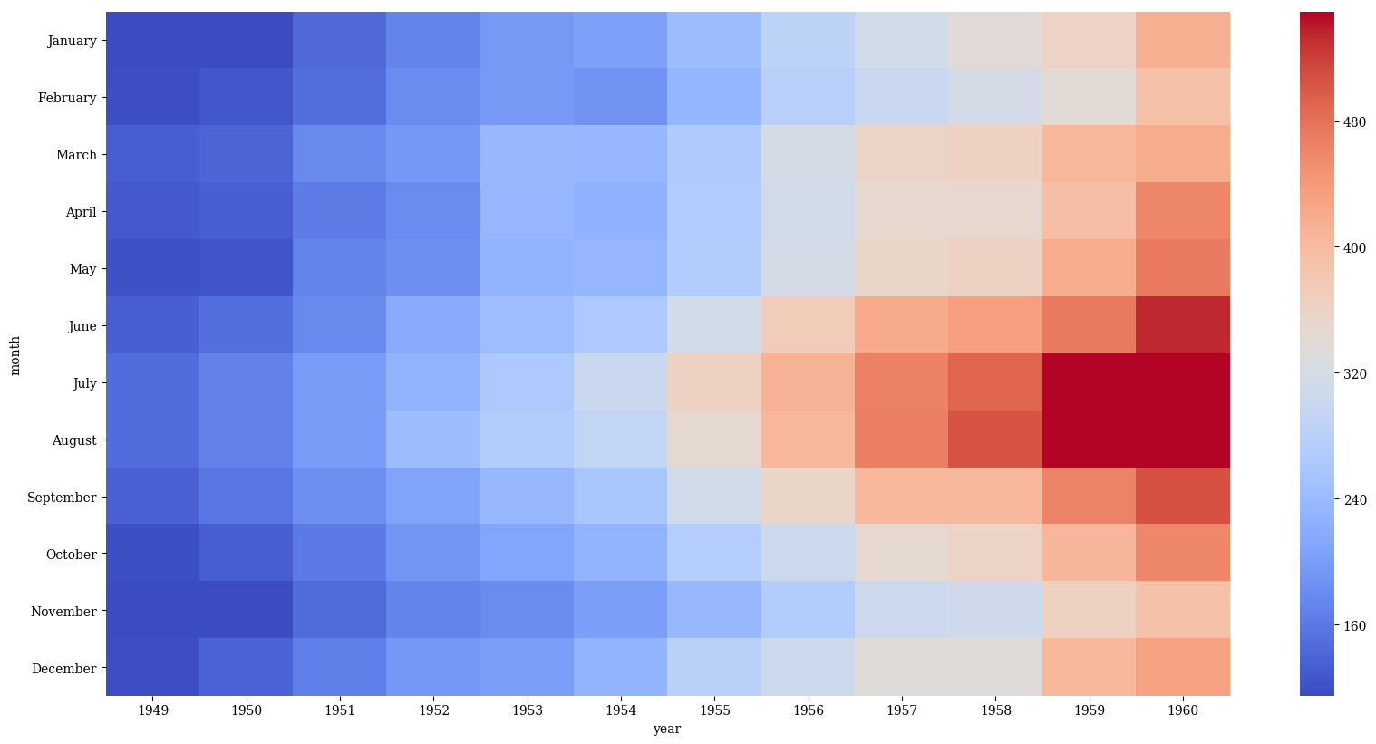
robust sets contrast levels based on quantiles and works like an “auto-contrast” for choosing good values

p = sns.heatmap(df, cmap='coolwarm', robust=True)

png

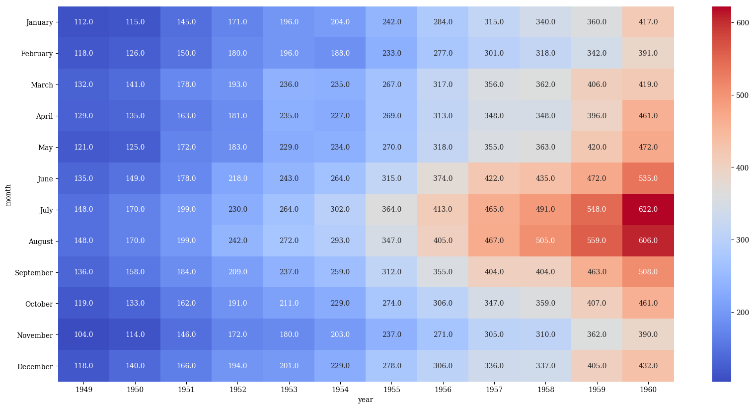
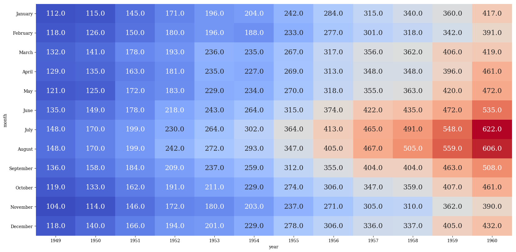
Label the rectangles with annot=True, which also chooses a suitable text color

p = sns.heatmap(df, cmap='coolwarm', annot=True)

png

The format of the annotation can be changed with fmt – here I’ll change from the default scientific notation to one decimal precision

p = sns.heatmap(df, cmap='coolwarm', annot=True, fmt=".1f")

png

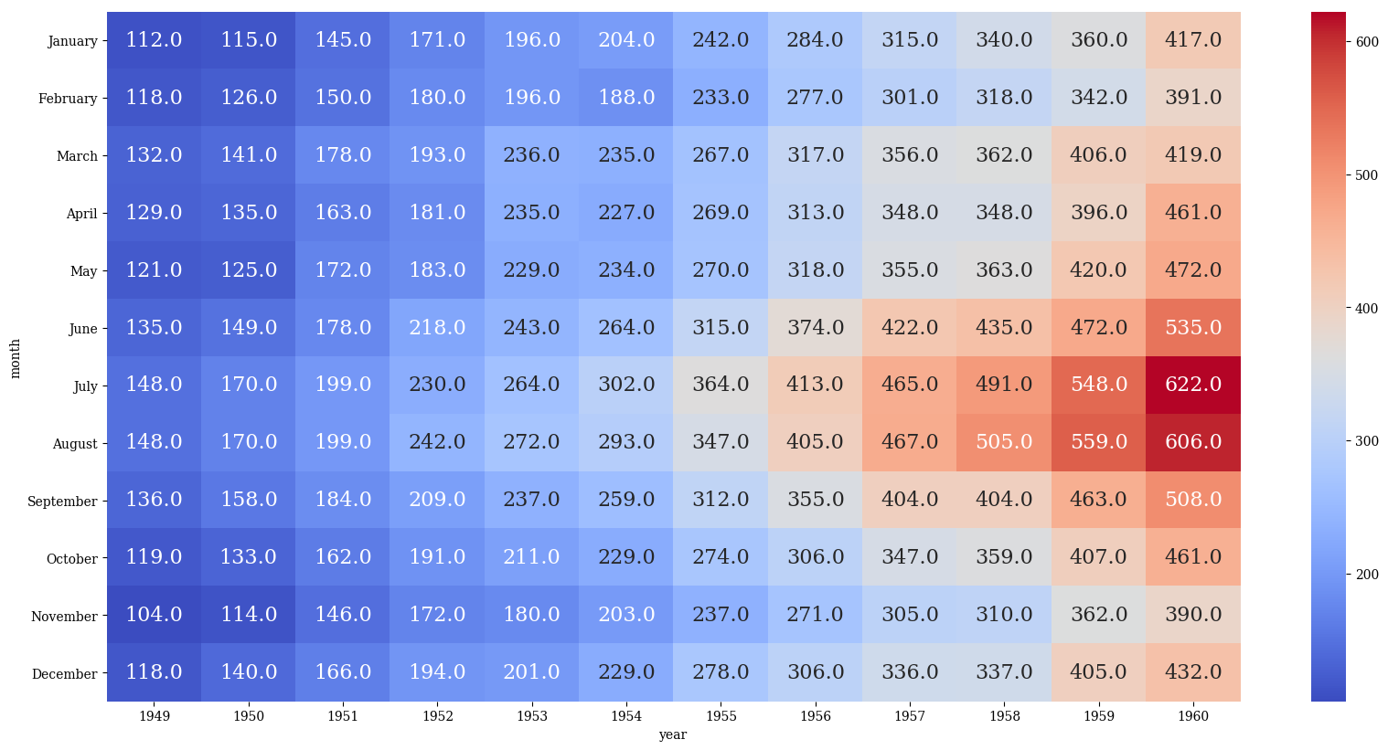
Any other parameters for the text, such as the font size, can be passed with annot_kws.

p = sns.heatmap(df, cmap='coolwarm', annot=True, fmt=".1f",annot_kws={'size':16})

png

cbar can be used to turn off the colorbar

p = sns.heatmap(df,
                cmap='coolwarm',
                annot=True,
                fmt=".1f",
                annot_kws={'size':16},
                cbar=False)

png

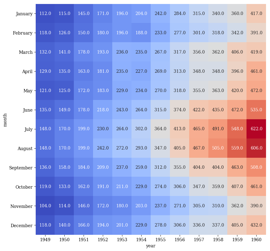
square forces the aspect ratio of the blocks to be equal

p = sns.heatmap(df,
                cmap='coolwarm',
                annot=True,
                fmt=".1f",
                annot_kws={'size':10},
                cbar=False,
                square=True)

png

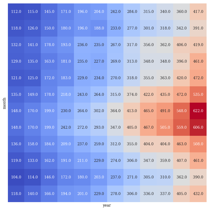
xticklabels and yticklabels are booleans to turn off the axis labels

p = sns.heatmap(df,
                cmap='coolwarm',
                annot=True,
                fmt=".1f",
                annot_kws={'size':10},
                cbar=False,
                square=True,
                xticklabels=False,
                yticklabels=False)

png

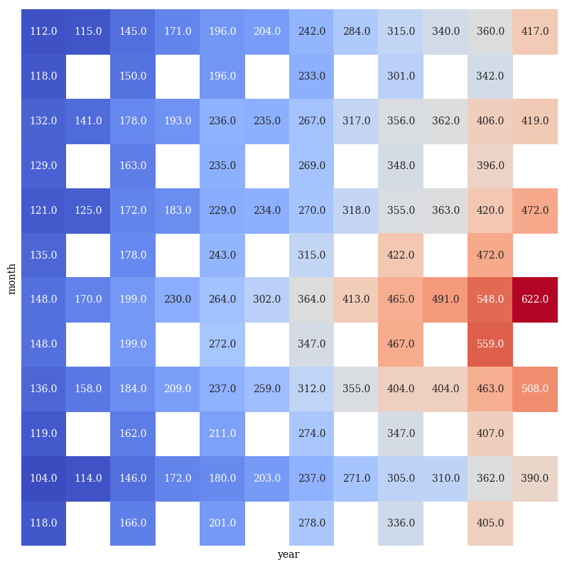
If you would like to hide certain values, pass in a binary mask

mask = np.zeros(df.shape)
mask[1::2,1::2] = 1
p = sns.heatmap(df,
                cmap='coolwarm',
                annot=True,
                fmt=".1f",
                annot_kws={'size':10},
                cbar=False,
                square=True,
                xticklabels=False,
                yticklabels=False,
                mask=mask)

png

Finalize

plt.rcParams['font.size'] = 20
bg_color = (0.88,0.85,0.95)
plt.rcParams['figure.facecolor'] = bg_color
plt.rcParams['axes.facecolor'] = bg_color
fig, ax = plt.subplots(1)
p = sns.heatmap(df,
                cmap='coolwarm',
                annot=True,
                fmt=".1f",
                annot_kws={'size':16},
                ax=ax)
plt.xlabel('Month')
plt.ylabel('Year')
ax.set_ylim((0,15))
plt.text(5,12.3, "Heat Map", fontsize = 95, color='Black', fontstyle='italic')

<matplotlib.text.Text at 0x10ec6acf8>

png

p.get_figure().savefig('../../figures/heatmap.png')