This is a detailed description of our solution to the Santander Product Recommendation competition hosted by Kaggle. The $60,000 challenge was to produce a recommendation system for Santander Banks, which is a global provider of a number of financial services. For this competition I teamed up with my good friend and fellow data scientist Matt – you can check out his blog here. We ended up placing 21st out of 1836 teams. I publicly released the code I used to clean the data in the form of Kaggle kernels early in the competition. You can view that either in Python or R. The full source code is also available on Github along with instructions for running it.
Overview
The goal of this competition was to take an approximately 13.6 million row dataset containing information about customers of Santander Banks between January 2015 and May 2016 and to predict which products they would purchase in June 2016, which was withheld from us. The purpose of this is so that Santander can build a better recommendation system and presumably do a better job of advertising services to the people that are likely to use them, not only saving Santander money, but also providing a better customer experience overall. Good all around. This is a bank, so the products are things like credit cards, debit accounts, payroll services, electronic banking, tax services, etc.
Specifically the challenge was to recommend the top 7 products to each customer. The scoring was evaluated using mean average precision at 7 (MAP@7). The intuition behind this scoring metric is that it rewards solutions where the person actually added one of the items you recommended, and you get more points if the purchased item was earlier in your list of recommendations. You don’t lose any points for recommending products to people that don’t buy anything. Therefore, you should recommend exactly 7 products to each customer, and place the most likely ones earlier in your list.
At a high level, a basic strategy for this kind of problem is the following. For each product, predict the probability that each customer will own it in the following month. These predictions can be the result of machine learning models, market basket analysis, etc. A list of recommended products can then be obtained by sorting these from most-likely to least-likely and removing the ones that are currently owned (remember, the task is to predict what they will own in addition to what they have now).
Solution Summary
Our recommendation system is based on gradient boosted classification trees. There are a number of machine learning software packages that implement this concept, but the most popular by far in the data science community, and the one we used here, is XGBoost. It’s really a fantastic piece of software that is fast, parallel, and supports extra features like L1/L2 regularization for the ensemble weights. At the time of this writing, XGBoost is used in more than half of winning solutions in machine learning competitions on Kaggle.
Gradient boosting is a machine learning strategy where you build many simple models that are called weak learners. Commonly these are decision trees, but the idea can be generalized to essentially any model. Each model you build focuses on the mistakes of the previous one(s), which is achieved by reweighting the input data to the ith weak learner based upon some error metric between the first i-1 models and the data. The output of the model as a whole is then a combination of the predictions made by each of the many weak learners.
Our final solution resulted from a blended ensemble average of predicted probabilities generated from a total of 100 different models, all XGBoost. These models were trained on various combinations of accounts in June 2015 and December 2015 that added products in that month. There were two primary modeling strategies:
-
Repeated single-class classification. A separate XGBoost model was trained for each product using
objective = "binary:logistic", and the target value was whether or not that product was owned, regardless of it being newly added or not. The result is that each set of predicted probabilities is the result of outputs from many models. The same input data was used for each of the sub-models. This method produced the best MAP@7 with a single model both for local cross-validation (CV) and on the public leaderboard. -
Multiclass classification. A single XGBoost model was trained using where the target variable was the product that was added. Using
objective = "multi:softprob", probabilities for each class were obtained all at once. For customers that added multiple products, a single one was chosen at random as the target.
Both types of models produce the probability that a customer will own or add each of the 22 products.
There were actually 24 products, but two of them, ind_aval_fin_ult1 and ind_ahor_fin_ult1, were discarded entirely
for being exceedingly rare.
A total of 5 separate models were built for each of the two above strategies using different combinations of features,
training data, and/or weightings, and each model was run with 10 different random seeds, resulting in the final total of 100 models.
The use of many different random seeds is to stabilize the predictions, and the probabilities across the 10 runs
for each model were combined with a flat average, reducing the total number of prediction sets from 100 to 10.
These 10 combined probabilties were then blended together using weights
that were tuned through a random search and optimized based upon the local CV MAP@7 of the resulting
recommendations (CV approach described below).
There were a couple of key insights that were critical to success in this competition. The first was limiting the dataset to only accounts that actually added any products. Note that the challenge is to predict which products a customer will add if any. We don’t need to determine the likelihood that they actually make the purchase, and any recommendations made to accounts that don’t purchase anything does not affect the score negatively. Adding products is a rare event and limiting only to entries where products were added reduces the dataset size from about 1 million entries per month to a much more reasonable 20-40,000.
Second, we found that the testing month, June, is special in Spain because that is when taxes are due. The result is that product purchase trends are quite different for June, particularly for tax services (d’oh). A helpful visualization of this was provided by Russ W. Training on data from June 2015 for accounts that added products with just the original features plus an additional one indicating whether or not each product was owned last month (which you need anyway to determine whether or not each product could have been added in the first place) produced a MAP@7 of ~0.027, which would have placed around top 35%.
The third realization was that the most useful features were those related to product ownership. After looking at the feature importance outputted by XGBoost, I added the product ownership status for each of the previous 2-5 months as features in addition to the most recent month and applied the repeated single-class classification strategy to produce a MAP@7 greater than 0.03 with a single model, which would have resulted in a top 100 finish and a bronze medal. These lagged ownership features were limited to 5 months because the earliest data was from January 2015 and thus this was the furthest back we could go. If I were actually being contracted by Santander to build a recommendation system, this is likely where I would have stopped. Estimates of the maximum possible score were around 0.035, so with this fairly simple approach we have already achieved more than 85% of the maximum possible precision. The additional time invested and model complexity added to slightly increase performance from public leaderboard MAP@7 of 0.03 to ~0.0306 (the difference in 15th and 150th place) was significant. But this is a competition so we pressed on.
The decision to train on December 2015 resulted from my trying to engineer more features related to product ownership. I figured there is a trade-off between 1) the advantage of capturing June-specific trends by training on June and 2) capturing product ownership trends by training on later months that have a longer history. I was in the process of exploring which months had similar purchasing patterns to June when Kaggler AMZ posted this analysis. He found December to be most similar to June and saved me some time, so many thanks to him for that. Training examples in December can contain up to 11 months of historical ownership features, the inclusion of which improved precision from 0.03 to ~0.0304 (roughly 150th to 40th place).
The addition of more features was enough to improve a single model to 0.0305. The 100 model ensemble then improved this to our final best public leaderboard score of 0.030599. As you can see, in this case ensembling added a lot of work for a very small gain. This was observed by other competitors, and the general consensus was that because mean average precision is evaluating a list of names rather than raw numbers, incremental improvements in probabilities that might make quite a difference if the evaluation metric was something like log loss don’t help rearrange the order of the recommendations very much.
Feature Engineering
The following features, mostly related to product ownership, were used and are listed in no particular order.
The features of type ownership were by far the most important. I’ve left the
Spanish names where applicable. Categorical features were one-hot encoded and converted to sparse matrices. Code for
producing all of these follows.
Base categorical features:
- sexo - gender
- ind_nuevo - is the customer new?
- ind_empleado - customer employee status
- segmento - segmentation
- nomprov - Province name
- indext - Foreigner index
- indresi - Residence index
- indrel - primary customer at beginning but not end of month
- tiprel_1mes - Customer relation type at the beginning of the month
- ind_actividad_cliente - customer active?
Base numerical features:
- age - age in years
- antiguedad - seniority in months
- renta - gross income
Engineered categorical features:
- ownership - binary feature indicating whether or not each product was owned 1-11 months ago (242 total features)
- owned.within - binary feature indicating whether or not each product was owned within 1-11 months ago (242 total features)
- segmento.change - is the value of
segmentodifferent last month than this month? - activity.index.change - is the value of
ind_actividad_clientedifferent last month than this month? - month - what is the current month?
- birthday.month - customer’s birthday month
Engineered numerical features:
- purchase.frequency - the number of times each product has been purchased (22 features)
- total_products - the total number of products owned 1-11 months ago (11 features)
- num.transactions - the total number of transaction 1-11 months ago (11 features). A transaction is defined as adding or dropping a product
- num.purchases - the total number of products added 1-11 months ago (11 features)
- months.since.owned - the number of months since each product was last owned (22 features)
Validation Strategy
The validation strategy changed depending on which methods were being used. Earlier in the competition, my strategy was to train on June 2015 only. Here, I split the data into a 75/25% train/test split, and computed the MAP@7 on the holdout. Another model was then trained using 100% of the training data and used to predict on the real testing data. I found local gains in MAP@7 for this method to be fairly consistent with gains on the public leaderboard.
When I switched to including December 2015 in the training data, I had to change strategies. The new CV method was to train on May 2015 and November 2015 and predict on May 2016. Here the CV performance was frustratingly quite inconsistent with the public scoring. June is a very different month, so features that may work well in some months might hurt in June, and vice versa. In addition, product purchase is a rare event, occurring only a few percent of the time. As the testing dataset contains about a million rows, only around 30,000 of them would be expected to make a purchase and thus potentially contribute to the score. Since the leaderboard is only computed on 30% of that, it means less than 10,000 accounts are contributing to the public scores, so there aren’t really that many samples. These two effects made it quite hard to gauge improvements, and resulted in myself, along with likely many others, trusting feedback from the public leaderboard more than local validation. Overfitting is of course a real danger here, but I didn’t see a way around it.
All hyperparameters for the models as well as the blending weights were optimized based upon this CV method.
Code Walkthrough
To start, we explore and clean the data.
Most of the following data cleaning and exploration sections were written by me at the very beginning of the competition when I was actually doing the exploration, and I have left the text mostly intact. Some approaches were changed later, such as the treatment of missing values, and I have added notes accordingly. Comments from future me are in italics
library(data.table)
library(dplyr)
library(tidyr)
library(lubridate)
library(ggplot2)
library(fasttime)
ggplot2 Theme Trick
A cool trick to avoid repetitive code in ggplot2 is to save/reuse your own theme. I’ll build one here and use it throughout.
my_theme <- theme_bw() +
  theme(axis.title=element_text(size=24),
        plot.title=element_text(size=36),
        axis.text =element_text(size=16))

my_theme_dark <- theme_dark() +
  theme(axis.title=element_text(size=24),
        plot.title=element_text(size=36),
        axis.text =element_text(size=16))
First Glance
setwd("~/kaggle/competition-santander/")
set.seed(1)
df   <- (fread("train_ver2.csv"))
##
Read 0.0% of 13647309 rows
Read 3.1% of 13647309 rows
Read 7.8% of 13647309 rows
Read 12.8% of 13647309 rows
Read 18.1% of 13647309 rows
Read 23.4% of 13647309 rows
Read 27.8% of 13647309 rows
Read 32.8% of 13647309 rows
Read 37.9% of 13647309 rows
Read 43.2% of 13647309 rows
Read 48.5% of 13647309 rows
Read 53.3% of 13647309 rows
Read 58.2% of 13647309 rows
Read 63.4% of 13647309 rows
Read 68.7% of 13647309 rows
Read 73.8% of 13647309 rows
Read 79.0% of 13647309 rows
Read 84.3% of 13647309 rows
Read 89.5% of 13647309 rows
Read 94.9% of 13647309 rows
Read 99.6% of 13647309 rows
Read 13647309 rows and 48 (of 48) columns from 2.135 GB file in 00:00:31
test <- (fread("test_ver2.csv"))
features <- names(df)[grepl("ind_+.*ult.*",names(df))]
I will create a label for each product and month that indicates whether a customer added, dropped or maintained that service in that billing cycle. I will do this by assigning a numeric id to each unique time stamp, and then matching each entry with the one from the previous month. The difference in the indicator value for each product then gives the desired value.
A cool trick to turn dates into unique id numbers is to use as.numeric(factor(...)). Make sure to order them chronologically first.
df                     <- df %>% arrange(fecha_dato) %>% as.data.table()
df$month.id            <- as.numeric(factor((df$fecha_dato)))
df$month.previous.id   <- df$month.id - 1
test$month.id          <- max(df$month.id) + 1
test$month.previous.id <- max(df$month.id)

# Test data will contain the status of products for the previous month, which is a feature. The training data currently contains the status of products as labels, and will later be joined to the previous month to get the previous month's ownership as a feature. I choose to do it in this order so that the train/test data can be cleaned together and then split. It's just for convenience.
test <- merge(test,df[,names(df) %in% c(features,"ncodpers","month.id"),with=FALSE],by.x=c("ncodpers","month.previous.id"),by.y=c("ncodpers","month.id"),all.x=TRUE)

df <- rbind(df,test)
We have a number of demographics for each individual as well as the products they currently own. To make a test set, I will separate the last month from this training data, and create a feature that indicates whether or not a product was newly purchased. First convert the dates. There’s fecha_dato, the row-identifier date, and fecha_alta, the date that the customer joined.
df[,fecha_dato:=fastPOSIXct(fecha_dato)]
df[,fecha_alta:=fastPOSIXct(fecha_alta)]
unique(df$fecha_dato)
##  [1] "2015-01-27 16:00:00 PST" "2015-02-27 16:00:00 PST"
##  [3] "2015-03-27 17:00:00 PDT" "2015-04-27 17:00:00 PDT"
##  [5] "2015-05-27 17:00:00 PDT" "2015-06-27 17:00:00 PDT"
##  [7] "2015-07-27 17:00:00 PDT" "2015-08-27 17:00:00 PDT"
##  [9] "2015-09-27 17:00:00 PDT" "2015-10-27 17:00:00 PDT"
## [11] "2015-11-27 16:00:00 PST" "2015-12-27 16:00:00 PST"
## [13] "2016-01-27 16:00:00 PST" "2016-02-27 16:00:00 PST"
## [15] "2016-03-27 17:00:00 PDT" "2016-04-27 17:00:00 PDT"
## [17] "2016-05-27 17:00:00 PDT" "2016-06-27 17:00:00 PDT"
I printed the values just to double check the dates were in standard Year-Month-Day format. I expect that customers will be more likely to buy products at certain months of the year (Christmas bonuses?), so let’s add a month column. I don’t think the month that they joined matters, so just do it for one.
df$month <- month(df$fecha_dato)
Are there any columns missing values?
sapply(df,function(x)any(is.na(x)))
##            fecha_dato              ncodpers          ind_empleado
##                 FALSE                 FALSE                 FALSE
##       pais_residencia                  sexo                   age
##                 FALSE                 FALSE                  TRUE
##            fecha_alta             ind_nuevo            antiguedad
##                  TRUE                  TRUE                  TRUE
##                indrel        ult_fec_cli_1t           indrel_1mes
##                  TRUE                 FALSE                  TRUE
##           tiprel_1mes               indresi                indext
##                 FALSE                 FALSE                 FALSE
##              conyuemp         canal_entrada               indfall
##                 FALSE                 FALSE                 FALSE
##               tipodom              cod_prov               nomprov
##                  TRUE                  TRUE                 FALSE
## ind_actividad_cliente                 renta              segmento
##                  TRUE                  TRUE                 FALSE
##     ind_ahor_fin_ult1     ind_aval_fin_ult1      ind_cco_fin_ult1
##                 FALSE                 FALSE                 FALSE
##     ind_cder_fin_ult1      ind_cno_fin_ult1     ind_ctju_fin_ult1
##                 FALSE                 FALSE                 FALSE
##     ind_ctma_fin_ult1     ind_ctop_fin_ult1     ind_ctpp_fin_ult1
##                 FALSE                 FALSE                 FALSE
##     ind_deco_fin_ult1     ind_deme_fin_ult1     ind_dela_fin_ult1
##                 FALSE                 FALSE                 FALSE
##     ind_ecue_fin_ult1     ind_fond_fin_ult1      ind_hip_fin_ult1
##                 FALSE                 FALSE                 FALSE
##     ind_plan_fin_ult1     ind_pres_fin_ult1     ind_reca_fin_ult1
##                 FALSE                 FALSE                 FALSE
##     ind_tjcr_fin_ult1     ind_valo_fin_ult1      ind_viv_fin_ult1
##                 FALSE                 FALSE                 FALSE
##       ind_nomina_ult1     ind_nom_pens_ult1       ind_recibo_ult1
##                  TRUE                  TRUE                 FALSE
##              month.id     month.previous.id                 month
##                 FALSE                 FALSE                 FALSE
Definitely. Onto data cleaning.
Data Cleaning
Going down the list, start with age
ggplot(data=df,aes(x=age)) +
  geom_bar(alpha=0.75,fill="tomato",color="black") +
  xlim(c(18,100)) +
  ggtitle("Age Distribution") +
  my_theme
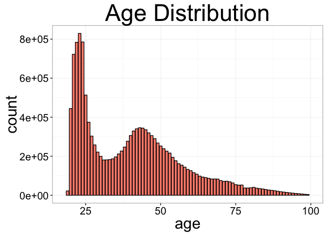
In addition to NA, there are people with very small and very high ages. It’s also interesting that the distribution is bimodal. There are a large number of university aged students, and then another peak around middle-age. Let’s separate the distribution and move the outliers to the mean of the closest one. I also add a feature indicating in which month the person’s birthday is – maybe you are more likely to add products then.
I later changed missing values to -1 as a flag and got slightly better results.
It seems some predictive power is contained in the lack of information itself. I also
later discovered that the first 6 months of this dataset appear to be backfilled and are stagnant.
For example, antiguedad (the number of months an account has existed) does not increment at all
for the first 6 months. Here I use the person’s birthday to backcorrect the ages. This might
seem like a small thing to do, but there is a harsh cutoff at age 20 for ownership of junior
accounts, so this little detail matters.
# df$age[(df$age < 18)] <- median(df$age[(df$age >= 18) & (df$age <=30)],na.rm=TRUE)
# df$age[(df$age > 100)] <- median(df$age[(df$age >= 30) & (df$age <=100)],na.rm=TRUE)
# df$age[is.na(df$age)] <- median(df$age,na.rm=TRUE)

age.change  <- df[month.id>6,.(age,month,month.id,age.diff=c(0,diff(age))),by="ncodpers"]
age.change  <- age.change[age.diff==1]
age.change  <- age.change[!duplicated(age.change$ncodpers)]
setkey(df,ncodpers)
df <- merge(df,age.change[,.(ncodpers,birthday.month=month)],by=c("ncodpers"),all.x=TRUE,sort=FALSE)
df$birthday.month[is.na(df$birthday.month)] <- 7 # July is the only month we don't get to check for increment so if there is no update then use it
df$age[df$birthday.month <= 7 & df$month.id<df$birthday.month] <- df$age[df$birthday.month <= 7 & df$month.id<df$birthday.month]  - 1 # correct ages in the first 6 months

df$age[is.na(df$age)] <- -1

df$age <- round(df$age)
I flip back and forth between dplyr and data.table, so sometimes you’ll see me casting things back and forth like this.
df <- as.data.frame(df)
Next ind_nuevo, which indicates whether a customer is new or not. How many missing values are there?
sum(is.na(df$ind_nuevo))
## [1] 27734
Let’s see if we can fill in missing values by looking how many months of history these customers have.
months.active <- df[is.na(df$ind_nuevo),] %>%
  group_by(ncodpers) %>%
  summarise(months.active=n())  %>%
  select(months.active)
max(months.active)
## [1] 6
Looks like these are all new customers, so replace accordingly.
df$ind_nuevo[is.na(df$ind_nuevo)] <- 1
Now, antiguedad
sum(is.na(df$antiguedad))
## [1] 27734
That number again. Probably the same people that we just determined were new customers. Double check.
summary(df[is.na(df$antiguedad),]%>%select(ind_nuevo))
##    ind_nuevo
##  Min.   :1
##  1st Qu.:1
##  Median :1
##  Mean   :1
##  3rd Qu.:1
##  Max.   :1
This feature is the number of months since the account joined and suffers
from the stagnation issue I mentioned previously in the first 6 months,
and here I correct it. Many customers have a valid value for fecha_alta,
the month that they joined, and this can be used to recompute antiguedad.
For entries without fecha_alta, I assume the value of antiguedad at month
6 is correct and correct the rest accordingly.
new.antiguedad <- df %>%
  dplyr::select(ncodpers,month.id,antiguedad) %>%
  dplyr::group_by(ncodpers) %>%
  dplyr::mutate(antiguedad=min(antiguedad,na.rm=T) + month.id - 6) %>% #month 6 is the first valid entry, so reassign based upon that reference
  ungroup() %>%
  dplyr::arrange(ncodpers) %>%
  dplyr::select(antiguedad)
df <- df %>%
  arrange(ncodpers) # arrange so that the two data frames are aligned
df$antiguedad <- new.antiguedad$antiguedad

df$antiguedad[df$antiguedad<0] <- -1

elapsed.months <- function(end_date, start_date) {
  12 * (year(end_date) - year(start_date)) + (month(end_date) - month(start_date))
}
recalculated.antiguedad <- elapsed.months(df$fecha_dato,df$fecha_alta)
df$antiguedad[!is.na(df$fecha_alta)] <- recalculated.antiguedad[!is.na(df$fecha_alta)]
df$ind_nuevo <- ifelse(df$antiguedad<=6,1,0) # reassign new customer index
Some entries don’t have the date they joined the company. Just give them something in the middle of the pack
df$fecha_alta[is.na(df$fecha_alta)] <- median(df$fecha_alta,na.rm=TRUE)
Next is indrel, which indicates:
1 (First/Primary), 99 (Primary customer during the month but not at the end of the month)
This sounds like a promising feature. I’m not sure if primary status is something the customer chooses or the company assigns, but either way it seems intuitive that customers who are dropping down are likely to have different purchasing behaviors than others.
table(df$indrel)
##
##        1       99
## 14522714    26476
Fill in missing with the more common status.
df$indrel[is.na(df$indrel)] <- 1
tipodom - Addres type. 1, primary address cod_prov - Province code (customer’s address)
tipodom doesn’t seem to be useful, and the province code is not needed becaue the name of the province exists in nomprov.
df <- df %>% select(-tipodom,-cod_prov)
Quick check back to see how we are doing on missing values
sapply(df,function(x)any(is.na(x)))
##              ncodpers            fecha_dato          ind_empleado
##                 FALSE                 FALSE                 FALSE
##       pais_residencia                  sexo                   age
##                 FALSE                 FALSE                 FALSE
##            fecha_alta             ind_nuevo            antiguedad
##                 FALSE                  TRUE                  TRUE
##                indrel        ult_fec_cli_1t           indrel_1mes
##                 FALSE                 FALSE                  TRUE
##           tiprel_1mes               indresi                indext
##                 FALSE                 FALSE                 FALSE
##              conyuemp         canal_entrada               indfall
##                 FALSE                 FALSE                 FALSE
##               nomprov ind_actividad_cliente                 renta
##                 FALSE                  TRUE                  TRUE
##              segmento     ind_ahor_fin_ult1     ind_aval_fin_ult1
##                 FALSE                 FALSE                 FALSE
##      ind_cco_fin_ult1     ind_cder_fin_ult1      ind_cno_fin_ult1
##                 FALSE                 FALSE                 FALSE
##     ind_ctju_fin_ult1     ind_ctma_fin_ult1     ind_ctop_fin_ult1
##                 FALSE                 FALSE                 FALSE
##     ind_ctpp_fin_ult1     ind_deco_fin_ult1     ind_deme_fin_ult1
##                 FALSE                 FALSE                 FALSE
##     ind_dela_fin_ult1     ind_ecue_fin_ult1     ind_fond_fin_ult1
##                 FALSE                 FALSE                 FALSE
##      ind_hip_fin_ult1     ind_plan_fin_ult1     ind_pres_fin_ult1
##                 FALSE                 FALSE                 FALSE
##     ind_reca_fin_ult1     ind_tjcr_fin_ult1     ind_valo_fin_ult1
##                 FALSE                 FALSE                 FALSE
##      ind_viv_fin_ult1       ind_nomina_ult1     ind_nom_pens_ult1
##                 FALSE                  TRUE                  TRUE
##       ind_recibo_ult1              month.id     month.previous.id
##                 FALSE                 FALSE                 FALSE
##                 month        birthday.month
##                 FALSE                 FALSE
Getting closer.
sum(is.na(df$ind_actividad_cliente))
## [1] 27734
By now you’ve probably noticed that this number keeps popping up. A handful of the entries are just bad, and should probably just be excluded from the model. But for now I will just clean/keep them.
I ultimately ended up keeping these entries and just kept the missing values separated
Just a couple more features.
df$ind_actividad_cliente[is.na(df$ind_actividad_cliente)] <- median(df$ind_actividad_cliente,na.rm=TRUE)
unique(df$nomprov)
##  [1] "MADRID"                 "BIZKAIA"
##  [3] "PALMAS, LAS"            "BURGOS"
##  [5] "CADIZ"                  "ALICANTE"
##  [7] "ZAMORA"                 "BARCELONA"
##  [9] "GIPUZKOA"               "GUADALAJARA"
## [11] ""                       "SEVILLA"
## [13] "GRANADA"                "CORUÑA, A"
## [15] "VALENCIA"               "BADAJOZ"
## [17] "CANTABRIA"              "MALAGA"
## [19] "ALMERIA"                "PONTEVEDRA"
## [21] "ALAVA"                  "GIRONA"
## [23] "AVILA"                  "MURCIA"
## [25] "SALAMANCA"              "SANTA CRUZ DE TENERIFE"
## [27] "SEGOVIA"                "JAEN"
## [29] "TOLEDO"                 "CACERES"
## [31] "NAVARRA"                "ASTURIAS"
## [33] "HUELVA"                 "LERIDA"
## [35] "LUGO"                   "ZARAGOZA"
## [37] "BALEARS, ILLES"         "PALENCIA"
## [39] "TARRAGONA"              "VALLADOLID"
## [41] "CIUDAD REAL"            "CASTELLON"
## [43] "OURENSE"                "RIOJA, LA"
## [45] "CORDOBA"                "ALBACETE"
## [47] "CUENCA"                 "HUESCA"
## [49] "LEON"                   "MELILLA"
## [51] "SORIA"                  "TERUEL"
## [53] "CEUTA"
There’s some rows missing a city that I’ll relabel
df$nomprov[df$nomprov==""] <- "UNKNOWN"
Now for gross income, aka renta
sum(is.na(df$renta))
## [1] 3022340
Here is a feature that is missing a lot of values. Rather than just filling them in with a median, it’s probably more accurate to break it down region by region. To that end, let’s take a look at the median income by region, and in the spirit of the competition let’s color it like the Spanish flag.
df %>%
  filter(!is.na(renta)) %>%
  group_by(nomprov) %>%
  summarise(med.income = median(renta)) %>%
  arrange(med.income) %>%
  mutate(city=factor(nomprov,levels=nomprov)) %>%
  ggplot(aes(x=city,y=med.income)) +
  geom_point(color="#c60b1e") +
  guides(color=FALSE) +
  xlab("City") +
  ylab("Median Income") +
  my_theme +
  theme(axis.text.x=element_blank(), axis.ticks = element_blank()) +
  geom_text(aes(x=city,y=med.income,label=city),angle=90,hjust=-.25) +
  theme(plot.background=element_rect(fill="#c60b1e"),
        panel.background=element_rect(fill="#ffc400"),
        panel.grid =element_blank(),
        axis.title =element_text(color="#ffc400"),
        axis.text  =element_text(color="#ffc400"),
        plot.title =element_text(color="#ffc400")) +
  ylim(c(60000,180000)) +


  ggtitle("Income Distribution by City")
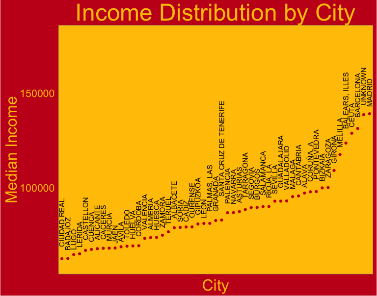
There’s a lot of variation, so I think assigning missing incomes by providence is a good idea. This code gets kind of confusing in a nested SQL statement kind of way, but the idea is to first group the data by city, and reduce to get the median. This intermediate data frame is joined by the original city names to expand the aggregated median incomes, ordered so that there is a 1-to-1 mapping between the rows, and finally the missing values are replaced.
Same story, I ended up not doing this and just treating missing values separately
# new.incomes <-df %>%
#   select(nomprov) %>%
#   merge(df %>%
#   group_by(nomprov) %>%
#   dplyr::summarise(med.income=median(renta,na.rm=TRUE)),by="nomprov") %>%
#   select(nomprov,med.income) %>%
#   arrange(nomprov)
# df <- arrange(df,nomprov)
# df$renta[is.na(df$renta)] <- new.incomes$med.income[is.na(df$renta)]
# rm(new.incomes)
#
# df$renta[is.na(df$renta)] <- median(df$renta,na.rm=TRUE)
df$renta[is.na(df$renta)] <- -1
The last line is to account for any values that are still missing. For example, it seems every entry from Alava has NA for renta.
The only remaining missing value are for features
sum(is.na(df$ind_nomina_ult1))
## [1] 16063
I could try to fill in missing values for products by looking at previous months, but since it’s such a small number of values for now I’ll take the cheap way out.
df[is.na(df)] <- 0
Now we have taken care of all the missing values. There’s also a bunch of character columns that can contain empty strings, so we need to go through them. For the most part, entries with empty strings will be converted to an unknown category.
str(df)
## 'data.frame':    14576924 obs. of  50 variables:
##  $ ncodpers             : int  15889 15889 15889 15889 15889 15889 15889 15889 15889 15889 ...
##  $ fecha_dato           : POSIXct, format: "2015-01-27 16:00:00" "2015-02-27 16:00:00" ...
##  $ ind_empleado         : chr  "F" "F" "F" "F" ...
##  $ pais_residencia      : chr  "ES" "ES" "ES" "ES" ...
##  $ sexo                 : chr  "V" "V" "V" "V" ...
##  $ age                  : num  55 55 55 55 55 55 56 56 56 56 ...
##  $ fecha_alta           : POSIXct, format: "1995-01-15 16:00:00" "1995-01-15 16:00:00" ...
##  $ ind_nuevo            : num  0 0 0 0 0 0 0 0 0 0 ...
##  $ antiguedad           : num  240 241 242 243 244 245 246 247 248 249 ...
##  $ indrel               : num  1 1 1 1 1 1 1 1 1 1 ...
##  $ ult_fec_cli_1t       : chr  "" "" "" "" ...
##  $ indrel_1mes          : chr  "1" "1" "1" "1" ...
##  $ tiprel_1mes          : chr  "A" "A" "A" "A" ...
##  $ indresi              : chr  "S" "S" "S" "S" ...
##  $ indext               : chr  "N" "N" "N" "N" ...
##  $ conyuemp             : chr  "N" "N" "N" "N" ...
##  $ canal_entrada        : chr  "KAT" "KAT" "KAT" "KAT" ...
##  $ indfall              : chr  "N" "N" "N" "N" ...
##  $ nomprov              : chr  "MADRID" "MADRID" "MADRID" "MADRID" ...
##  $ ind_actividad_cliente: num  1 1 1 1 1 1 1 1 1 1 ...
##  $ renta                : num  326125 326125 326125 326125 326125 ...
##  $ segmento             : chr  "01 - TOP" "01 - TOP" "01 - TOP" "01 - TOP" ...
##  $ ind_ahor_fin_ult1    : int  0 0 0 0 0 0 0 0 0 0 ...
##  $ ind_aval_fin_ult1    : int  0 0 0 0 0 0 0 0 0 0 ...
##  $ ind_cco_fin_ult1     : int  1 1 1 1 1 1 1 1 1 1 ...
##  $ ind_cder_fin_ult1    : int  0 0 0 0 0 0 0 0 0 0 ...
##  $ ind_cno_fin_ult1     : int  0 0 0 0 0 0 0 0 0 0 ...
##  $ ind_ctju_fin_ult1    : int  0 0 0 0 0 0 0 0 0 0 ...
##  $ ind_ctma_fin_ult1    : int  0 0 0 0 0 0 0 0 0 0 ...
##  $ ind_ctop_fin_ult1    : int  0 0 0 0 0 0 0 0 0 0 ...
##  $ ind_ctpp_fin_ult1    : int  1 1 1 1 1 1 1 1 1 1 ...
##  $ ind_deco_fin_ult1    : int  0 0 0 0 0 0 0 0 0 0 ...
##  $ ind_deme_fin_ult1    : int  0 0 0 0 0 0 0 0 0 0 ...
##  $ ind_dela_fin_ult1    : int  0 0 0 0 0 0 0 0 0 0 ...
##  $ ind_ecue_fin_ult1    : int  0 0 0 0 0 0 0 0 0 0 ...
##  $ ind_fond_fin_ult1    : int  0 0 0 0 0 0 0 0 0 0 ...
##  $ ind_hip_fin_ult1     : int  0 0 0 0 0 0 0 0 0 0 ...
##  $ ind_plan_fin_ult1    : int  0 0 0 0 0 0 0 0 0 0 ...
##  $ ind_pres_fin_ult1    : int  0 0 0 0 0 0 0 0 0 0 ...
##  $ ind_reca_fin_ult1    : int  0 0 0 0 0 0 0 0 0 0 ...
##  $ ind_tjcr_fin_ult1    : int  1 0 0 0 1 1 1 0 0 0 ...
##  $ ind_valo_fin_ult1    : int  1 1 1 1 1 1 1 1 1 1 ...
##  $ ind_viv_fin_ult1     : int  0 0 0 0 0 0 0 0 0 0 ...
##  $ ind_nomina_ult1      : num  0 0 0 0 0 0 0 0 0 0 ...
##  $ ind_nom_pens_ult1    : num  0 0 0 0 0 0 0 0 0 0 ...
##  $ ind_recibo_ult1      : int  0 0 0 0 0 0 0 0 0 0 ...
##  $ month.id             : num  1 2 3 4 5 6 7 8 9 10 ...
##  $ month.previous.id    : num  0 1 2 3 4 5 6 7 8 9 ...
##  $ month                : num  1 2 3 4 5 6 7 8 9 10 ...
##  $ birthday.month       : num  7 7 7 7 7 7 7 7 7 7 ...
char.cols <- names(df)[sapply(df,is.character)]
for (name in char.cols){
  print(sprintf("Unique values for %s:", name))
  print(unique(df[[name]]))
  }
## [1] "Unique values for ind_empleado:"
## [1] "F" "A" "N" "B" ""  "S"
## [1] "Unique values for pais_residencia:"
##   [1] "ES" ""   "PT" "NL" "AD" "IN" "VE" "US" "FR" "GB" "IT" "DE" "MX" "CL"
##  [15] "CO" "CH" "CR" "PE" "JP" "AT" "AR" "AE" "BE" "MA" "CI" "QA" "SE" "BR"
##  [29] "FI" "RS" "KE" "JM" "RU" "AU" "CU" "EC" "KR" "DO" "LU" "GH" "CZ" "PA"
##  [43] "IE" "BO" "CM" "CA" "GR" "ZA" "RO" "KH" "IL" "NG" "CN" "DK" "NZ" "MM"
##  [57] "SG" "UY" "NI" "EG" "GI" "PH" "KW" "VN" "TH" "NO" "GQ" "BY" "AO" "UA"
##  [71] "TR" "PL" "OM" "GA" "GE" "BG" "HR" "PR" "HK" "HN" "BA" "MD" "HU" "SK"
##  [85] "TN" "TG" "SA" "MR" "DZ" "LB" "MT" "SV" "PK" "PY" "LY" "MK" "EE" "SN"
##  [99] "MZ" "GT" "GN" "TW" "IS" "LT" "CD" "KZ" "BZ" "CF" "GM" "ET" "SL" "GW"
## [113] "LV" "CG" "ML" "BM" "ZW" "AL" "DJ"
## [1] "Unique values for sexo:"
## [1] "V" "H" ""
## [1] "Unique values for ult_fec_cli_1t:"
##   [1] ""           "2015-08-05" "2016-03-17" "2015-12-04" "2016-03-29"
##   [6] "2015-07-15" "2016-04-12" "2015-12-17" "2015-10-27" "2016-04-19"
##  [11] "2016-05-24" "2015-07-03" "2016-02-23" "2016-05-30" "2015-10-05"
##  [16] "2015-07-27" "2016-02-24" "2015-12-03" "2015-11-16" "2015-12-01"
##  [21] "2016-05-17" "2015-09-29" "2016-01-26" "2016-01-05" "2016-05-20"
##  [26] "2015-11-12" "2016-03-02" "2016-04-01" "2016-03-16" "2015-07-22"
##  [31] "2016-06-23" "2015-12-09" "2015-10-13" "2016-03-18" "2015-11-11"
##  [36] "2015-11-10" "2015-08-20" "2015-08-03" "2015-08-19" "2015-10-06"
##  [41] "2016-05-02" "2015-10-02" "2016-02-11" "2015-07-20" "2016-05-27"
##  [46] "2015-07-21" "2016-06-01" "2016-03-04" "2016-04-22" "2015-12-11"
##  [51] "2015-09-08" "2015-12-15" "2016-04-15" "2015-07-28" "2016-02-08"
##  [56] "2016-05-26" "2015-12-02" "2015-09-10" "2015-11-27" "2016-06-24"
##  [61] "2015-10-21" "2015-08-24" "2015-12-28" "2015-11-02" "2016-01-19"
##  [66] "2016-01-18" "2016-03-15" "2015-07-17" "2016-01-22" "2015-09-01"
##  [71] "2015-08-18" "2015-10-22" "2015-07-07" "2016-03-28" "2015-09-21"
##  [76] "2016-01-13" "2016-02-16" "2015-09-23" "2015-11-23" "2016-06-28"
##  [81] "2015-12-10" "2015-12-24" "2015-11-24" "2016-05-09" "2016-02-01"
##  [86] "2016-04-06" "2015-10-28" "2016-05-18" "2016-01-28" "2015-08-13"
##  [91] "2016-04-05" "2016-02-15" "2015-09-15" "2015-10-01" "2015-10-20"
##  [96] "2016-02-09" "2016-03-23" "2015-07-06" "2016-03-14" "2016-04-07"
## [101] "2016-01-11" "2016-06-03" "2016-02-12" "2015-07-14" "2015-09-11"
## [106] "2015-09-03" "2016-01-21" "2016-02-04" "2016-06-06" "2015-12-16"
## [111] "2015-11-19" "2015-08-06" "2015-12-21" "2015-08-27" "2015-11-18"
## [116] "2016-04-26" "2016-05-12" "2015-07-01" "2016-01-15" "2015-08-14"
## [121] "2016-02-25" "2015-09-14" "2016-03-07" "2016-01-12" "2016-04-08"
## [126] "2015-12-30" "2015-11-17" "2016-06-07" "2016-01-08" "2016-06-14"
## [131] "2015-08-25" "2015-09-28" "2015-09-24" "2016-06-22" "2016-01-07"
## [136] "2015-11-13" "2016-06-27" "2016-03-11" "2015-09-25" "2015-08-28"
## [141] "2015-11-25" "2016-01-25" "2016-05-06" "2015-08-04" "2015-08-10"
## [146] "2015-09-22" "2015-10-26" "2016-04-21" "2016-01-04" "2016-03-08"
## [151] "2015-12-14" "2015-09-18" "2016-05-25" "2016-03-10" "2016-03-01"
## [156] "2016-02-10" "2016-06-17" "2016-05-05" "2015-08-17" "2015-10-15"
## [161] "2016-06-10" "2015-11-04" "2015-10-07" "2016-06-21" "2015-09-02"
## [166] "2016-04-20" "2015-08-21" "2016-05-23" "2015-11-03" "2016-05-04"
## [171] "2015-07-30" "2015-07-09" "2015-10-19" "2016-05-10" "2015-07-29"
## [176] "2016-04-14" "2015-08-26" "2015-09-04" "2016-02-02" "2016-06-08"
## [181] "2015-12-22" "2016-02-26" "2015-10-09" "2015-09-17" "2016-01-27"
## [186] "2016-02-22" "2016-06-09" "2016-03-22" "2015-10-08" "2015-12-18"
## [191] "2016-02-03" "2016-03-30" "2016-04-28" "2016-04-13" "2016-06-15"
## [196] "2016-06-13" "2016-01-20" "2015-11-05" "2015-12-29" "2016-04-18"
## [201] "2016-06-16" "2015-07-02" "2015-11-20" "2016-04-27" "2015-12-07"
## [206] "2015-11-06" "2016-05-03" "2015-07-13" "2016-02-17" "2015-10-14"
## [211] "2015-08-11" "2015-10-29" "2016-06-20" "2016-04-04" "2016-02-18"
## [216] "2016-06-29" "2015-07-10" "2015-07-16" "2015-07-23" "2015-10-23"
## [221] "2016-05-19" "2016-05-11" "2015-12-23" "2015-11-26" "2015-11-09"
## [226] "2016-04-11" "2016-03-09" "2015-08-12" "2015-07-08" "2015-09-07"
## [231] "2016-03-21" "2015-09-09" "2016-01-14" "2015-09-16" "2016-03-24"
## [236] "2015-10-16" "2016-02-19" "2016-04-25" "2016-06-02" "2016-02-05"
## [241] "2016-05-16" "2016-03-03" "2016-05-13" "2015-08-07" "2015-07-24"
## [1] "Unique values for indrel_1mes:"
##  [1] "1"   "2"   "1.0" "2.0" "4.0" ""    "3.0" "3"   "P"   "4"   "0"
## [1] "Unique values for tiprel_1mes:"
## [1] "A" "I" "P" ""  "R" "N"
## [1] "Unique values for indresi:"
## [1] "S" ""  "N"
## [1] "Unique values for indext:"
## [1] "N" "S" ""
## [1] "Unique values for conyuemp:"
## [1] "N" "S" ""
## [1] "Unique values for canal_entrada:"
##   [1] "KAT" "013" "KFA" ""    "KFC" "KAS" "007" "KHK" "KCH" "KHN" "KHC"
##  [12] "KFD" "RED" "KAW" "KHM" "KCC" "KAY" "KBW" "KAG" "KBZ" "KBO" "KEL"
##  [23] "KCI" "KCG" "KES" "KBL" "KBQ" "KFP" "KEW" "KAD" "KDP" "KAE" "KAF"
##  [34] "KAA" "KDO" "KEY" "KHL" "KEZ" "KAH" "KAR" "KHO" "KHE" "KBF" "KBH"
##  [45] "KAO" "KFV" "KDR" "KBS" "KCM" "KAC" "KCB" "KAL" "KGX" "KFT" "KAQ"
##  [56] "KFG" "KAB" "KAZ" "KGV" "KBJ" "KCD" "KDU" "KAJ" "KEJ" "KBG" "KAI"
##  [67] "KBM" "KDQ" "KAP" "KDT" "KBY" "KAM" "KFK" "KFN" "KEN" "KDZ" "KCA"
##  [78] "KHQ" "KFM" "004" "KFH" "KFJ" "KBR" "KFE" "KDX" "KDM" "KDS" "KBB"
##  [89] "KFU" "KAV" "KDF" "KCL" "KEG" "KDV" "KEQ" "KAN" "KFL" "KDY" "KEB"
## [100] "KGY" "KBE" "KDC" "KBU" "KAK" "KBD" "KEK" "KCF" "KED" "KAU" "KEF"
## [111] "KFR" "KCU" "KCN" "KGW" "KBV" "KDD" "KCV" "KBP" "KCT" "KBN" "KCX"
## [122] "KDA" "KCO" "KCK" "KBX" "KDB" "KCP" "KDE" "KCE" "KEA" "KDG" "KDH"
## [133] "KEU" "KFF" "KEV" "KEC" "KCS" "KEH" "KEI" "KCR" "KDW" "KEO" "KHS"
## [144] "KFS" "025" "KFI" "KHD" "KCQ" "KDN" "KHR" "KEE" "KEM" "KFB" "KGU"
## [155] "KCJ" "K00" "KDL" "KDI" "KGC" "KHA" "KHF" "KGN" "KHP"
## [1] "Unique values for indfall:"
## [1] "N" "S" ""
## [1] "Unique values for nomprov:"
##  [1] "MADRID"                 "BIZKAIA"
##  [3] "PALMAS, LAS"            "BURGOS"
##  [5] "CADIZ"                  "ALICANTE"
##  [7] "ZAMORA"                 "BARCELONA"
##  [9] "GIPUZKOA"               "GUADALAJARA"
## [11] "UNKNOWN"                "SEVILLA"
## [13] "GRANADA"                "CORUÑA, A"
## [15] "VALENCIA"               "BADAJOZ"
## [17] "CANTABRIA"              "MALAGA"
## [19] "ALMERIA"                "PONTEVEDRA"
## [21] "ALAVA"                  "GIRONA"
## [23] "AVILA"                  "MURCIA"
## [25] "SALAMANCA"              "SANTA CRUZ DE TENERIFE"
## [27] "SEGOVIA"                "JAEN"
## [29] "TOLEDO"                 "CACERES"
## [31] "NAVARRA"                "ASTURIAS"
## [33] "HUELVA"                 "LERIDA"
## [35] "LUGO"                   "ZARAGOZA"
## [37] "BALEARS, ILLES"         "PALENCIA"
## [39] "TARRAGONA"              "VALLADOLID"
## [41] "CIUDAD REAL"            "CASTELLON"
## [43] "OURENSE"                "RIOJA, LA"
## [45] "CORDOBA"                "ALBACETE"
## [47] "CUENCA"                 "HUESCA"
## [49] "LEON"                   "MELILLA"
## [51] "SORIA"                  "TERUEL"
## [53] "CEUTA"
## [1] "Unique values for segmento:"
## [1] "01 - TOP"           "02 - PARTICULARES"  ""
## [4] "03 - UNIVERSITARIO"
Okay, based on that and the definitions of each variable, I will fill the empty strings either with the most common value or create an unknown category based on what I think makes more sense.
df$indfall[df$indfall==""]                 <- "N"
df$tiprel_1mes[df$tiprel_1mes==""]         <- "A"
df$indrel_1mes[df$indrel_1mes==""]         <- "1"
df$indrel_1mes[df$indrel_1mes=="P"]        <- "5"
df$indrel_1mes <- as.factor(as.integer(df$indrel_1mes))

df$pais_residencia[df$pais_residencia==""] <- "UNKNOWN"
df$sexo[df$sexo==""]                       <- "UNKNOWN"
df$ult_fec_cli_1t[df$ult_fec_cli_1t==""]   <- "UNKNOWN"
df$ind_empleado[df$ind_empleado==""]       <- "UNKNOWN"
df$indext[df$indext==""]                   <- "UNKNOWN"
df$indresi[df$indresi==""]                 <- "UNKNOWN"
df$conyuemp[df$conyuemp==""]               <- "UNKNOWN"
df$segmento[df$segmento==""]               <- "UNKNOWN"
Convert all the features to numeric dummy indicators (you’ll see why in a second), and we’re done cleaning
features <- grepl("ind_+.*ult.*",names(df))
df[,features] <- lapply(df[,features],function(x)as.integer(round(x)))
Lag Features
Very important to this competition were so-called lag features, meaning that for each entry
it was beneficial to consider not only the value of a feature for the current month, but
also the value for previous months. Soon after discovering that lagged product ownership was a
useful feature (i.e. whether or not a product was owned 1,2,3,4,etc months ago), I figured it
was possible to use other lagged features. Here is a function that makes it easy to create such
features. The idea is to join the data by account id, ncodpers, and to match the month with the
lag month. For example, to add a 2-month lag feature to an observation in month 5, we want to extract
the value of feature.name at month 3.
# create-lag-feature.R

create.lag.feature <- function(dt, # should be a data.table!
                               feature.name, # name of the feature to lag
                               months.to.lag=1,# vector of integers indicating how many months to lag
                               by=c("ncodpers","month.id"), # keys to join data.tables by
                               na.fill = NA)
  {
  # get the feature and change the name to avoid .x and .y being appending to names
  dt.sub <- dt[,mget(c(by,feature.name))]
  names(dt.sub)[names(dt.sub) == feature.name] <- "original.feature"
  original.month.id <- dt.sub$month.id
  added.names <- c()
  for (month.ago in months.to.lag){
    print(paste("Collecting information on",feature.name,month.ago,"month(s) ago"))
    colname <- paste("lagged.",feature.name,".",month.ago,"months.ago",sep="")
    added.names <- c(colname,added.names)
    # This is a self join except the month is shifted
    dt.sub <- merge(dt.sub,
                    dt.sub[,.(ncodpers,
                              month.id=month.ago+original.month.id,
                              lagged.feature=original.feature)],
                    by=by,
                    all.x=TRUE,
                    sort=FALSE)
    names(dt.sub)[names(dt.sub)=="lagged.feature"] <- colname
    # dt.sub[[colname]][is.na(dt.sub[[colname]])] <- dt.sub[["original.feature"]][is.na(dt.sub[[colname]])]
  }
  df <- merge(dt,
              dt.sub[,c(by,added.names),with=FALSE],
              by=by,
              all.x=TRUE,
              sort=FALSE)
  df[is.na(df)] <- na.fill
  return(df)
}
Now I use that function to create lagged features of ind_actividad_cliente, the customer activity index. For a few percent of customers I noticed that ind_actividad_cliente was almost perfectly correlated with one of a few products (particularly ind_tjcr_fin_ult1 (credit card), ind_cco_fin_ult1 (current accounts), and ind_recibo_ult1 (debit account)). I think this is actually a leak in the dataset, as it appears such a customer was marked as active because they used a product. Therefore, I thought this was going to be an extremely powerful feature, but it turned out to not provide much, if any, benefit. My conclusion was that although this was a useful predictor for that few percent of customers, the problem is being unable to identify which accounts followed this trend. To me it seems ind_actividad_cliente is recorded with high inconsistency. Some customers own many products and are marked inactive, while others are marked active but own nothing. Maybe one of the teams who outperformed us figured out how to utilize this information.
source('project/Santander/lib/create-lag-feature.R')
df <- as.data.table(df)
df <- create.lag.feature(df,'ind_actividad_cliente',1:11,na.fill=0)
## [1] "Collecting information on ind_actividad_cliente 1 month(s) ago"
## [1] "Collecting information on ind_actividad_cliente 2 month(s) ago"
## [1] "Collecting information on ind_actividad_cliente 3 month(s) ago"
## [1] "Collecting information on ind_actividad_cliente 4 month(s) ago"
## [1] "Collecting information on ind_actividad_cliente 5 month(s) ago"
## [1] "Collecting information on ind_actividad_cliente 6 month(s) ago"
## [1] "Collecting information on ind_actividad_cliente 7 month(s) ago"
## [1] "Collecting information on ind_actividad_cliente 8 month(s) ago"
## [1] "Collecting information on ind_actividad_cliente 9 month(s) ago"
## [1] "Collecting information on ind_actividad_cliente 10 month(s) ago"
## [1] "Collecting information on ind_actividad_cliente 11 month(s) ago"
Junior accounts, ind_ctju_fin_ult1, are for those 19 and younger. I found that the month that a customer turned 20 there was a discontinuation of ind_ctju_fin_ult1 followed by a high likelihood of adding e-accounts, ind_ecue_fin_ult1. I add a binary feature to capture this.
df[,last.age:=lag(age),by="ncodpers"]
df$turned.adult <- ifelse(df$age==20 & df$last.age==19,1,0)
df <- as.data.frame(df)
Now the data is cleaned, separate it back into train/test. I’m writing a csv file because I will do some other analysis that uses these files, but if you are ever just saving variables to use them again in R you should write binary files with save and load – they are way faster.
features <- names(df)[grepl("ind_+.*ult.*",names(df))]

test <- df %>%
  filter(month.id==max(df$month.id))
df <- df %>%
  filter(month.id<max(df$month.id))
write.csv(df,"cleaned_train.csv",row.names=FALSE)
write.csv(test,"cleaned_test.csv",row.names=FALSE)
Data Visualization
These are some of the plots I made at the beginning of the competition to get a sense of what the data was like and to get preliminary ideas for features. I will say, however, that most of the useful insights ultimately came from a combination of XGBoost feature importance outputs and from going through the raw data for many accounts by hand.
To study trends in customers adding or removing services, I will create a label for each product and month that indicates whether a customer added, dropped or maintained that service in that billing cycle. I will do this by assigning a numeric id to each unique time stamp, and then matching each entry with the one from the previous month. The difference in the indicator value for each product then gives the desired value.
A cool trick to turn dates into unique id numbers is to use as.numeric(factor(...)). Make sure to order them chronologically first.
features          <- grepl("ind_+.*ult.*",names(df))
df[,features]     <- lapply(df[,features],function(x)as.integer(round(x)))
df$total.services <- rowSums(df[,features],na.rm=TRUE)
df                <- df %>% arrange(fecha_dato)
df$month.id       <- as.numeric(factor((df$fecha_dato)))
df$month.next.id  <- df$month.id + 1
Now I’ll build a function that will convert differences month to month into a meaningful label. Each month, a customer can either maintain their current status with a particular product, add it, or drop it.
status.change <- function(x){
  if ( length(x) == 1 ) { # if only one entry exists, I'll assume they are a new customer and therefore are adding services
    label = ifelse(x==1,"Added","Maintained")
  } else {
    diffs <- diff(x) # difference month-by-month
    diffs <- c(0,diffs) # first occurrence will be considered Maintained, which is a little lazy. A better way would be to check if the earliest date was the same as the earliest we have in the dataset and consider those separately. Entries with earliest dates later than that have joined and should be labeled as "Added"
    label <- rep("Maintained", length(x))
    label <- ifelse(diffs==1,"Added",
                    ifelse(diffs==-1,"Dropped",
                           "Maintained"))
  }
  label
}
Now we can actually apply this function to each feature using lapply and ave
df[,features] <- lapply(df[,features], function(x) return(ave(x,df$ncodpers, FUN=status.change)))
I’m only interested in seeing what influences people adding or removing services, so I’ll trim away any instances of “Maintained”. Since big melting/casting operations can be slow, I’ll take the time to check for rows that should be completely removed, then melt the remainder and remove the others.
interesting <- rowSums(df[,features]!="Maintained")
df          <- df[interesting>0,]
df          <- df %>%
                gather(key=feature,
                value=status,
                ind_ahor_fin_ult1:ind_recibo_ult1)
df          <- filter(df,status!="Maintained")
head(df)
##   ncodpers month.id          fecha_dato ind_empleado pais_residencia sexo
## 1    53273        2 2015-02-27 16:00:00            N              ES    V
## 2   352884        4 2015-04-27 17:00:00            N              ES    H
## 3   507549        4 2015-04-27 17:00:00            N              ES    V
## 4   186769        5 2015-05-27 17:00:00            N              ES    V
## 5   186770        5 2015-05-27 17:00:00            N              ES    H
## 6   110663        6 2015-06-27 17:00:00            N              ES    V
##   age          fecha_alta ind_nuevo antiguedad indrel ult_fec_cli_1t
## 1  42 2000-04-05 17:00:00         0        178      1        UNKNOWN
## 2  41 2002-04-21 17:00:00         0        156      1        UNKNOWN
## 3  49 2004-12-19 16:00:00         0        124      1        UNKNOWN
## 4  49 2000-08-02 17:00:00         0        177      1        UNKNOWN
## 5  46 2000-08-02 17:00:00         0        177      1        UNKNOWN
## 6  38 2002-06-16 17:00:00         0        156      1        UNKNOWN
##   indrel_1mes tiprel_1mes indresi indext conyuemp canal_entrada indfall
## 1           1           A       S      N  UNKNOWN           KAT       N
## 2           1           A       S      N  UNKNOWN           KAT       N
## 3           1           I       S      N  UNKNOWN           KAT       N
## 4           1           A       S      N  UNKNOWN           KAT       N
## 5           1           A       S      N  UNKNOWN           KAT       N
## 6           1           A       S      N  UNKNOWN           KAT       N
##                  nomprov ind_actividad_cliente    renta          segmento
## 1              BARCELONA                     1 121920.3          01 - TOP
## 2             VALLADOLID                     1  60303.3 02 - PARTICULARES
## 3 SANTA CRUZ DE TENERIFE                     0  99163.8 02 - PARTICULARES
## 4                 MADRID                     1     -1.0          01 - TOP
## 5                 MADRID                     1     -1.0 02 - PARTICULARES
## 6                 MADRID                     1 395567.8 02 - PARTICULARES
##   month.previous.id month birthday.month
## 1                 1     2              6
## 2                 3     4              2
## 3                 3     4              1
## 4                 4     5              1
## 5                 4     5              9
## 6                 5     6              9
##   lagged.ind_actividad_cliente.11months.ago
## 1                                         0
## 2                                         0
## 3                                         0
## 4                                         0
## 5                                         0
## 6                                         0
##   lagged.ind_actividad_cliente.10months.ago
## 1                                         0
## 2                                         0
## 3                                         0
## 4                                         0
## 5                                         0
## 6                                         0
##   lagged.ind_actividad_cliente.9months.ago
## 1                                        0
## 2                                        0
## 3                                        0
## 4                                        0
## 5                                        0
## 6                                        0
##   lagged.ind_actividad_cliente.8months.ago
## 1                                        0
## 2                                        0
## 3                                        0
## 4                                        0
## 5                                        0
## 6                                        0
##   lagged.ind_actividad_cliente.7months.ago
## 1                                        0
## 2                                        0
## 3                                        0
## 4                                        0
## 5                                        0
## 6                                        0
##   lagged.ind_actividad_cliente.6months.ago
## 1                                        0
## 2                                        0
## 3                                        0
## 4                                        0
## 5                                        0
## 6                                        0
##   lagged.ind_actividad_cliente.5months.ago
## 1                                        0
## 2                                        0
## 3                                        0
## 4                                        0
## 5                                        0
## 6                                        1
##   lagged.ind_actividad_cliente.4months.ago
## 1                                        0
## 2                                        0
## 3                                        0
## 4                                        1
## 5                                        1
## 6                                        1
##   lagged.ind_actividad_cliente.3months.ago
## 1                                        0
## 2                                        1
## 3                                        0
## 4                                        1
## 5                                        1
## 6                                        1
##   lagged.ind_actividad_cliente.2months.ago
## 1                                        0
## 2                                        1
## 3                                        0
## 4                                        1
## 5                                        1
## 6                                        1
##   lagged.ind_actividad_cliente.1months.ago last.age turned.adult
## 1                                        1       42            0
## 2                                        1       41            0
## 3                                        0       49            0
## 4                                        1       49            0
## 5                                        1       46            0
## 6                                        1       38            0
##   total.services month.next.id           feature  status
## 1              6             3 ind_ahor_fin_ult1   Added
## 2              4             5 ind_ahor_fin_ult1 Dropped
## 3              0             5 ind_ahor_fin_ult1 Dropped
## 4              8             6 ind_ahor_fin_ult1 Dropped
## 5              6             6 ind_ahor_fin_ult1 Dropped
## 6              2             7 ind_ahor_fin_ult1 Dropped
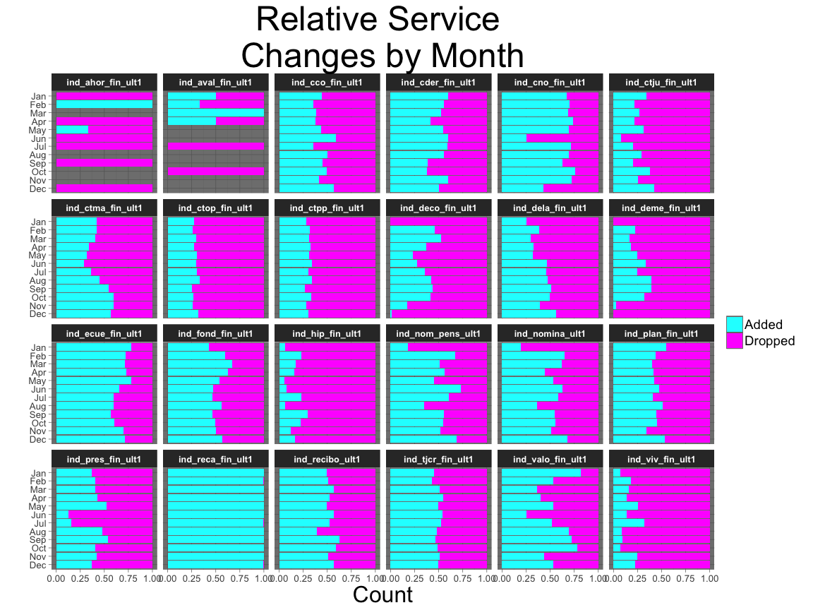
Does the ratio of dropping/adding services change over the year?
totals.by.feature <- df %>%
  group_by(month,feature) %>%
  summarise(counts=n())

df %>%
  group_by(month,feature,status) %>%
  summarise(counts=n())%>%
  ungroup() %>%
  inner_join(totals.by.feature,by=c("month","feature")) %>%

  mutate(counts=counts.x/counts.y) %>%
  ggplot(aes(y=counts,x=factor(month.abb[month],levels=month.abb[seq(12,1,-1)]))) +
  geom_bar(aes(fill=status), stat="identity") +
  facet_wrap(facets=~feature,ncol = 6) +
  coord_flip() +
  my_theme_dark +
  ylab("Count") +
  xlab("") +
  ylim(limits=c(0,1)) +
  ggtitle("Relative Service \nChanges by Month") +
  theme(axis.text   = element_text(size=10),
        legend.text = element_text(size=14),
        legend.title= element_blank()      ,
        strip.text  = element_text(face="bold")) +
  scale_fill_manual(values=c("cyan","magenta"))
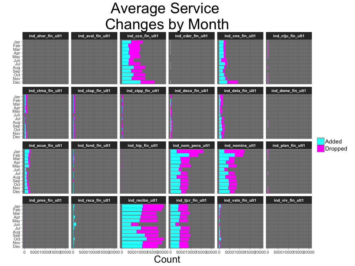
Let’s see how product changes vary over the calendar year. Some months occur more than others, so we need to account for that.
month.counts              <- table(unique(df$month.id)%%12)
cur.names                 <- names(month.counts)
cur.names[cur.names=="0"] <- "12"
names(month.counts) <- cur.names
month.counts              <- data.frame(month.counts) %>%
  rename(month=Var1,month.count=Freq) %>% mutate(month=as.numeric(month))

df %>%
  group_by(month,feature,status) %>%
  summarise(counts=n())%>%
  ungroup() %>%
  inner_join(month.counts,by="month") %>%

  mutate(counts=counts/month.count) %>%
  ggplot(aes(y=counts,x=factor(month.abb[month],levels=month.abb[seq(12,1,-1)]))) +
  geom_bar(aes(fill=status), stat="identity") +
  facet_wrap(facets=~feature,ncol = 6) +
  coord_flip() +
  my_theme_dark +
  ylab("Count") +
  xlab("") +
  ggtitle("Average Service \nChanges by Month") +
  theme(axis.text    = element_text(size=10),
        legend.text  = element_text(size=14),
        legend.title = element_blank()      ,
        strip.text   = element_text(face="bold")) +
  scale_fill_manual(values=c("cyan","magenta"))
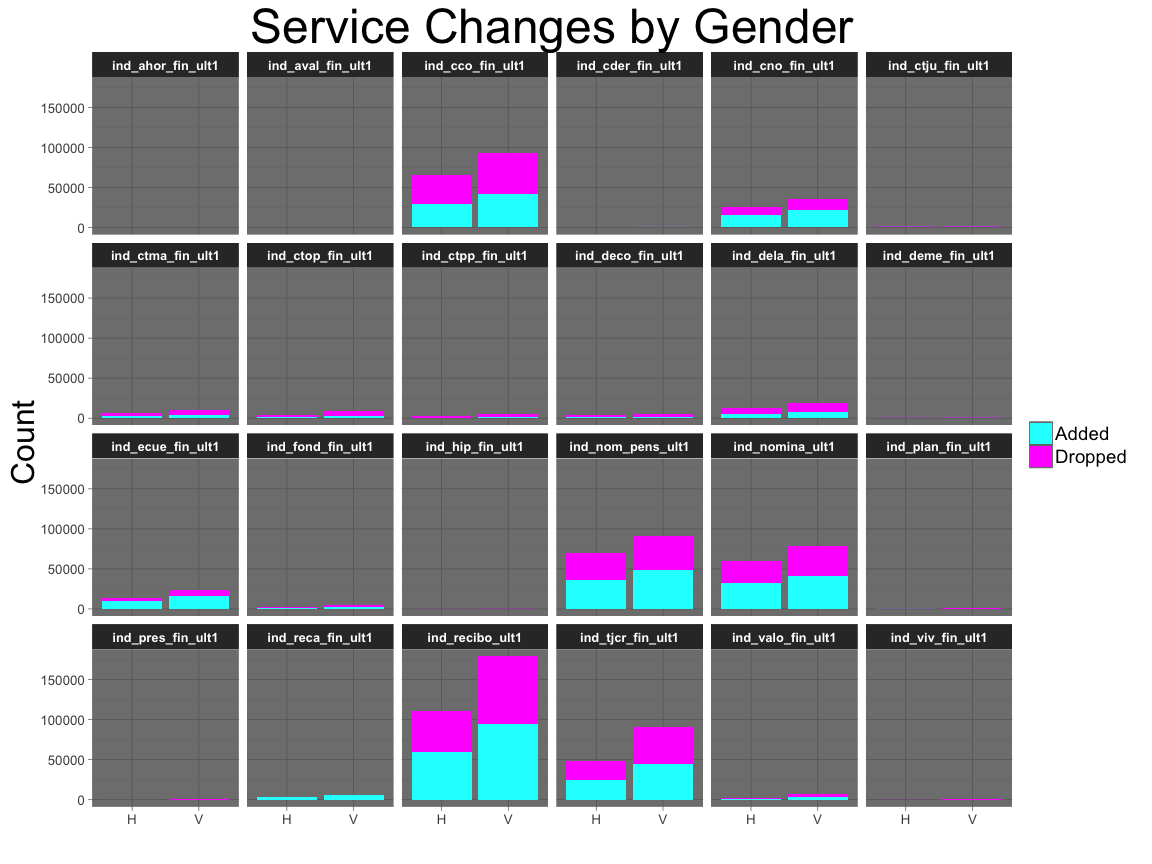
df %>%
  filter(sexo!="UNKNOWN") %>%
  ggplot(aes(x=sexo)) +
  geom_bar(aes(fill=status)) +
  facet_wrap(facets=~feature,ncol = 6) +
  my_theme_dark +
  ylab("Count") +
  xlab("") +
  ggtitle("Service Changes by Gender") +
  theme(axis.text    = element_text(size=10),
        legend.text  = element_text(size=14),
        legend.title = element_blank()      ,
        strip.text   = element_text(face="bold")) +
  scale_fill_manual(values=c("cyan","magenta"))
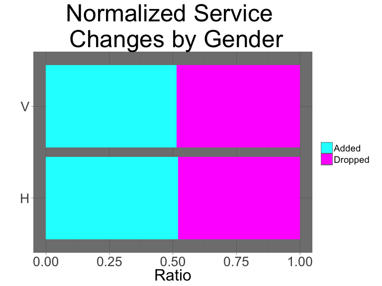
tot.H  <- sum(df$sexo=="H")
tot.V  <- sum(df$sexo=="V")
tmp.df <- df %>%
  group_by(sexo,status) %>%
  summarise(counts=n())
tmp.df$counts[tmp.df$sexo=="H"] = tmp.df$counts[tmp.df$sexo=="H"] / tot.H
tmp.df$counts[tmp.df$sexo=="V"] = tmp.df$counts[tmp.df$sexo=="V"] / tot.V
tmp.df %>%
  filter(sexo!="UNKNOWN") %>%
  ggplot(aes(x=factor(feature),y=counts)) +
  geom_bar(aes(fill=status,sexo),stat='identity') +
  coord_flip() +
  my_theme_dark +
  ylab("Ratio") +
  xlab("") +
  ggtitle("Normalized Service \n Changes by Gender") +
  theme(axis.text    = element_text(size=20),
        legend.text  = element_text(size=14),
        legend.title = element_blank()      ,
        strip.text   = element_text(face="bold")) +
  scale_fill_manual(values=c("cyan","magenta"))
rm(tmp.df)
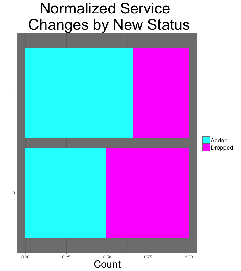
tot.new     <- sum(df$ind_nuevo==1)
tot.not.new <- sum(df$ind_nuevo!=1)
tmp.df      <- df %>%
  group_by(ind_nuevo,status) %>%
  summarise(counts=n())
tmp.df$counts[tmp.df$ind_nuevo==1] = tmp.df$counts[tmp.df$ind_nuevo==1] / tot.new
tmp.df$counts[tmp.df$ind_nuevo!=1] = tmp.df$counts[tmp.df$ind_nuevo!=1] / tot.not.new
tmp.df %>%
  ggplot(aes(x=factor(feature),y=counts)) +
  geom_bar(aes(fill=status,factor(ind_nuevo)),stat='identity') +
  coord_flip() +
  my_theme_dark +
  ylab("Count") +
  xlab("") +
  ggtitle("Normalized Service \n Changes by New Status") +
  theme(axis.text    = element_text(size=10),
        legend.text  = element_text(size=14),
        legend.title = element_blank()      ,
        strip.text   = element_text(face="bold")) +
  scale_fill_manual(values=c("cyan","magenta"))
rm(tmp.df)
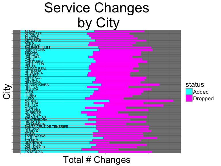
df %>%
  group_by(nomprov,status) %>%
  summarise(y=mean(total.services)) %>%
  ggplot(aes(x=factor(nomprov,levels=sort(unique(nomprov),decreasing=TRUE)),y=y)) +
  geom_bar(stat="identity",aes(fill=status)) +
  geom_text(aes(label=nomprov),
            y=0.2,
            hjust=0,
            angle=0,
            size=3,
            color="#222222") +
  coord_flip() +
  my_theme_dark +
  xlab("City") +
  ylab("Total # Changes") +
  ggtitle("Service Changes\n by City") +
  theme(axis.text    = element_blank(),
        legend.text  = element_text(size=14),
        legend.title = element_text(size=18)) +
  scale_fill_manual(values=c("cyan","magenta"))
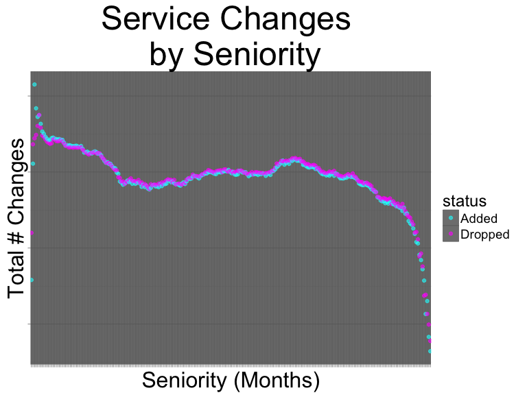
df %>%
  group_by(antiguedad,status) %>%
  summarise(counts=n()) %>%
  ggplot(aes(x=factor(antiguedad),y=log(counts))) +
  geom_point(alpha=0.6,aes(color=status)) +
  my_theme_dark +
  xlab("Seniority (Months)") +
  ylab("Total # Changes") +
  ggtitle("Service Changes \n by Seniority") +
  theme(axis.text    = element_blank(),
        legend.text  = element_text(size=14),
        legend.title = element_text(size=18)) +
  scale_color_manual(values=c("cyan","magenta"))
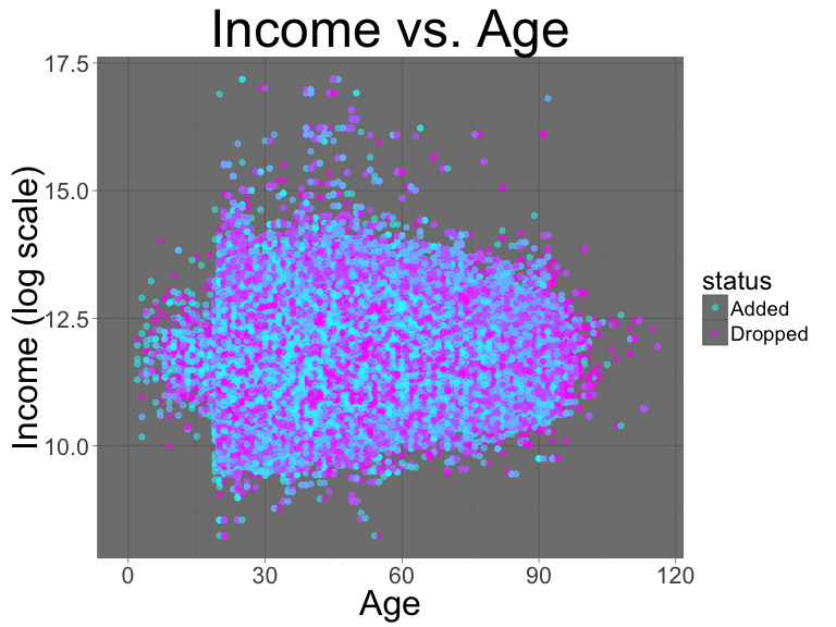
df %>%
  ggplot(aes(x=age,y=log(renta))) +
  geom_point(alpha=0.5,aes(color=status)) +
  my_theme_dark +
  xlab("Age") +
  ylab("Income (log scale)") +
  ggtitle("Income vs. Age") +
  theme(
        legend.text  = element_text(size=14),
        legend.title = element_text(size=18)) +
  scale_color_manual(values=c("cyan","magenta"))
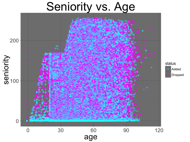
df %>%
  group_by(ncodpers) %>%
  slice(c(1,n())) %>%
  select(age,seniority=antiguedad,status) %>%
  ggplot(aes(x=age,y=seniority)) +
  geom_point(alpha=0.4,aes(color=status)) +
  ggtitle("Seniority vs. Age") +
  my_theme_dark +
  scale_color_manual(values=c("cyan","magenta"))
df %>%
  group_by(nomprov,status) %>%
  summarise(y=mean(total.services)) %>%
  ggplot(aes(x=factor(nomprov,levels=sort(unique(nomprov),decreasing=TRUE)),y=y)) +
  geom_bar(stat="identity",aes(fill=status)) +
  geom_text(aes(label=nomprov),
            y=0.2,
            hjust=0,
            angle=0,
            size=3,
            color="#222222") +
  coord_flip() +
  my_theme_dark +
  xlab("City") +
  ylab("Total # Changes") +
  ggtitle("Service Changes\n by City") +
  theme(axis.text    = element_blank(),
        legend.text  = element_text(size=14),
        legend.title = element_text(size=18)) +
  scale_fill_manual(values=c("cyan","magenta"))

Feature Engineering
Here is a description of the features and how they were made
List of purchased products
We need a list of the products each customer purchased each month so that we can compute the MAP@7 on our validation set. This can be done by connecting each row to the corresponding one from the previous month. If the difference in the product’s ownership status now and one month ago is equal to 1, then that product was added and we append it to our list.
## create-purchased-column.R
# This script outputs a csv file containing a list of new products purchased
# each month by each customer.
library(data.table)
# setwd('~/kaggle/competition-santander/')
df     <- fread("cleaned_train.csv")
labels <- names(df)[grepl("ind_+.*_+ult",names(df))]
cols   <- c("ncodpers","month.id","month.previous.id",labels)
df     <- df[,names(df) %in% cols,with=FALSE]

# connect each month to the previous one
df     <- merge(df,df,by.x=c("ncodpers","month.previous.id"),by.y=c("ncodpers","month.id"),all.x=TRUE)

# entries that don't have a corresponding row for the previous month will be NA and
# I will treat these as if that product was owned
df[is.na(df)] <- 0

# for each product, the difference between the current month on the left and the
# previous month on the right indicates whether a product was added (+1), dropped (-1),
# or unchanged (0)
products <- rep("",nrow(df))
for (label in labels){
  colx  <- paste0(label,".x")
  coly  <- paste0(label,".y")
  diffs <- df[,.(get(colx)-get(coly))]
  products[diffs>0] <- paste0(products[diffs>0],label,sep=" ")
}

# write results
df <- df[,.(ncodpers,month.id,products)]
write.csv(df,"purchased-products.csv",row.names=FALSE)
MAP@k
The code used to calculate MAP@k came from Kaggle
apk <- function(k, actual, predicted)
{
  if (length(actual)==0){return(0.0)}
  score <- 0.0
  cnt <- 0.0
  for (i in 1:min(k,length(predicted)))
  {
    if (predicted[i] %in% actual && !(predicted[i] %in% predicted[0:(i-1)]))
    {
      cnt   <- cnt + 1
      score <- score + cnt/i
    }
  }
  score <- score / min(length(actual), k)
  if (is.na(score)){
    debug<-0
  }
  return(score)
}

mapk <- function (k, actual, predicted)
{
  if( length(actual)==0 || length(predicted)==0 )
  {
    return(0.0)
  }

  scores <- rep(0, length(actual))
  for (i in 1:length(scores))
  {
    scores[i] <- apk(k, actual[[i]], predicted[[i]])
  }
  score <- mean(scores)
  score
}
Frequency of product purchase and number of transactions by month
The purchase frequency is a feature indicating number of times the customer has added each product. This is obtained
by getting the product change status and cumulatively summing the positive changes, which
indicate product addition. These values are on an absolute scale – customers that have
been around longer have more time to acquire large values for these features. To me, it seems
like it would be more important to capture the purchase frequency per month. For example, many
customers frequency add and drop ind_tjcr_fin_ult1 (credit card). I think this just means
the customer only uses the credit card intermittently, so the ownership status flips on/off
frequently month-to-month. If we compare two such customers, one who had a long history with the bank
and another with a short one, the one who had been around longer would have built up more
product purchases. But we really want this behavior of sporadic ownership to be captured
simultaneously. To that end, I tried normalizing the purchase frequency by the number of months that the
customer had been a member (basically you assign an index df[,idx:=1:.N,by=”ncodpers”] and then
divide the purchase frequency by that index); however, this actually hurt the resulting score.
In the end, I left it as an absolute scale as follows.
## feature-purchase-frequency.R

library(data.table)
# setwd('~/kaggle/competition-santander/')
df     <- fread("cleaned_train.csv")
labels <- names(df)[grepl("ind_+.*_+ult",names(df))]
cols   <- c("ncodpers","month.id","month.previous.id",labels)
df     <- df[,names(df) %in% cols,with=FALSE]
df     <- merge(df,df,by.x=c("ncodpers","month.previous.id"),by.y=c("ncodpers","month.id"),all.x=TRUE)

df[is.na(df)] <- 0
products <- rep("",nrow(df))
num.transactions <- rep(0,nrow(df))
purchase.frequencies <- data.frame(ncodpers=df$ncodpers, month.id=(df$month.previous.id + 2))
for (label in labels){
  colx  <- paste0(label,".x") # x column is the left data frame and contains more recent information
  coly  <- paste0(label,".y")
  diffs <- df[,.(ncodpers,month.id,change=get(colx)-get(coly))]
  # num.transactions counts the number of adds and drops
  num.transactions <- num.transactions + as.integer(diffs$change!=0)
  diffs[diffs<0] <- 0 # only consider positive cases for the purchase frequency
  setkey(diffs,ncodpers)
  d <- diffs[,.(frequency = cumsum(change)),by=ncodpers]
  purchase.frequencies[[paste(label,"_purchase.count",sep="")]] <- d$frequency

}
purchase.frequencies$num.transactions <- num.transactions
purchase.frequencies <- purchase.frequencies %>%
  dplyr::group_by(ncodpers) %>%
  dplyr::mutate(num.transactions = cumsum(num.transactions))
write.csv(purchase.frequencies,"purchase.frequencies.csv",row.names=FALSE)
Number of months since product was last owned
This function calculates how many months have passed since the product was last owned, defaulting to 999 if there is no prior ownership. By the time this function is called in the model, there are boolean features of the form <product name>_#month_ago indicating whether or not the corresponding product was owned # months ago. Starting with the furthest month back, we update the ownership vector with the current temporal distance at the positions where the product was owned that month. By doing it this way, the last time a particular position is updated will be correspond to the last time it was owned. Suppose account X owns product Y for months 1-5 and then drops it, and then for an observation in month 12 we wish to know how many months since Y was owned, searching 11 months total. 11 months ago was month 1, and the product was owned, so we record an 11. That continues until we look 7 months ago at month 5, and record 7 months for the feature value. When we look 6 months ago at month 6, the product was not owned, and we don’t do anything. The final value of the feature will 7, the number of months since X owned Y.
# months-since-owned.R

months.since.owned<- function(dt,products,months.to.search,default.value = 999){

  for (product in products){
      print(paste("Finding months since owning",product))
      colname <- paste(product,".last.owned",sep="")
      dt[[colname]] <- default.value
    for (month.ago in seq(months.to.search,1,-1)){
      cur.colname <- paste(product,"_",month.ago,"month_ago",sep="")
      dt[[colname]][dt[[cur.colname]] == 1] <- month.ago
    }
  }
  return(dt)

}
The following is the main script that does feature engineering and produces the data ready (mostly) to be fed into one of the models
# engineer-features.R

setwd("~/kaggle/competition-santander/")
library(tidyr)
library(xgboost)
library(plyr)
library(dplyr)
library(data.table)
library(ggplot2)
library(caret)
library(pROC)
library(lubridate)
library(fasttime)
source('project/Santander/lib/get_recommendations.R')
source('project/Santander/lib/MAP.R')
source("project/Santander/lib/months-since-owned.R")

set.seed(1)
# Train on month 5 and 11 and validate on 17 for CV data then
# train on month 6 and 12 and predict on test. The second months are separated
# into a separate variable so I can turn on/off using them
val.train.month <- 5
val.test.month  <- 17
train.month     <- 6
extra.train.months.val <- c(11)
extra.train.months.test <- c(12)

months.to.keep  <- c(val.train.month,val.test.month,train.month,extra.train.months.val,extra.train.months.test)
df   <- fread("cleaned_train.csv")
test <- fread("cleaned_test.csv")

# add activity index previous month
recent.activity.index <- merge(rbind(df[,.(ncodpers,month.id,ind_actividad_cliente,
                                     segmento)],
                                     test[,.(ncodpers,month.id,ind_actividad_cliente,
                                           segmento)]),
                               df[,.(ncodpers,month.id=month.id+1,
                                     old.ind_actividad_cliente=ind_actividad_cliente,
                                     old.segmento=segmento)],
                               by=c("ncodpers","month.id"),
                               sort=FALSE)
                               # all.x=TRUE) # might not want all.x here, means people that weren't customers last month will be considered to change activity
recent.activity.index[,activity.index.change:=ind_actividad_cliente-old.ind_actividad_cliente]
recent.activity.index[,segmento.change:=as.integer(segmento!=old.segmento)]
df   <- merge(df,recent.activity.index[,.(ncodpers,
                                          month.id,
                                          old.ind_actividad_cliente,
                                          activity.index.change,
                                          old.segmento,
                                          segmento.change)],
              by=c("ncodpers","month.id"),all.x=TRUE)

test <- merge(test,recent.activity.index[,.(ncodpers,
                                            month.id,
                                            old.ind_actividad_cliente,
                                            activity.index.change,
                                            old.segmento,
                                            segmento.change)],
              by=c("ncodpers","month.id"),all.x=TRUE)

df$old.segmento[is.na(df$old.segmento)] <- df$segmento[is.na(df$old.segmento)]
df$ind_actividad_cliente[is.na(df$ind_actividad_cliente)] <- df$old.ind_actividad_cliente[is.na(df$ind_actividad_cliente)]

df[is.na(df)] <- 0

products <- names(df)[grepl("ind_+.*_+ult",names(df))]

# create a data frame with just the product ownership variables so we can create lag ownership features
products.owned <- df %>%
  select(ncodpers,month.id,one_of(products)) %>%
  as.data.table()

df   <- as.data.table(df)
test <- as.data.table(test)
original.month.id <- products.owned$month.id
df <- df[month.id %in% months.to.keep,]


test <- test[,!names(test) %in% products,with=FALSE] #lazy, but I'm removing product ownership because it is about to be readded month by month

# create features indicating whether or not a product was owned in each of the past
# X months. for each lag, match the month with the earlier one and through some name manipulation
# extract whether the product was owned or not
for (month.ago in 1:11){
  print(paste("Collecting data on product ownership",month.ago,"months ago..."))
  products.owned[,month.id:=original.month.id+month.ago]
  df <- merge(df,products.owned,by=c("ncodpers","month.id"),all.x=TRUE)
  change.names <- names(df)[grepl("\\.y",names(df))]
  new.names <- gsub("\\.y",paste("_",month.ago,"month_ago",sep=""),change.names)
  names(df)[grepl("\\.y",names(df))] <- new.names

  #I'm being lazy here...
  change.names <- names(df)[grepl("\\.x",names(df))]
  new.names <- gsub("\\.x","",change.names)
  names(df)[grepl("\\.x",names(df))] <- new.names


  test <- merge(test,products.owned,by=c("ncodpers","month.id"),all.x=TRUE)

  change.names <- names(test)[grepl("\\.y",names(test))]
  new.names <- gsub("\\.y",paste("_",month.ago,"month_ago",sep=""),change.names)
  names(test)[grepl("\\.y",names(test))] <- new.names

  change.names <- names(test)[grepl("\\.x",names(test))]
  new.names <- gsub("\\.x","",change.names)
  names(test)[grepl("\\.x",names(test))] <- new.names

}
names(test)[names(test) %in% products] <- paste(names(test)[names(test) %in% products],"_1month_ago",sep="")

# there will be NA values where there isn't a match to the left side since we used all.x=TRUE, assume those correspond
# to products that were not owned
df[is.na(df)] <- 0
test[is.na(test)] <- 0

# get the number of months since each product was owned
df <- months.since.owned(df,products,12)
test <- months.since.owned(test,products,12)
df <- as.data.frame(df)
test <- as.data.frame(test)


# compute total number of products owned previous month
df$total_products <- rowSums(df[,names(df) %in% names(df)[grepl("ind.*1month\\_ago",names(df))]],na.rm=TRUE)
test$total_products <- rowSums(test[,names(test) %in% names(test)[grepl("ind.*1month\\_ago",names(test))]],na.rm=TRUE)

# save the month id for use creating window ownership features
products.owned$month.id <- original.month.id

# windows of product ownership. For each window size look back at previous months and see if the product was
# ever owned. I do this by adding the value of the ownership variable X months ago for X = 1:window.size
# then converting to a binary indicator if the value is positive (meaning it was owned at least once)
 for (product in products){
   for (window.size in 2:6){
     print(paste("Getting ownership for",product,"within last",window.size,"months"))
     colname <- paste(product,".owned.within.",window.size,"months",sep="")
     df[[colname]]   <- 0
     test[[colname]] <- 0
     for (month.ago in 1:window.size){
      current.col     <- paste(product,"_",month.ago,"month_ago",sep="")
      df[[colname]]   <- df[[colname]]  + df[[current.col]]
      test[[colname]] <- test[[colname]]  + test[[current.col]]
     }
     df[[colname]]   <- as.integer(df[[colname]] > 0)
     test[[colname]] <- as.integer(test[[colname]] > 0)
   }
 }

# add in purchase frequency feature for each product
purchase.frequencies <- fread("purchase.frequencies.csv")

df   <- merge(df,purchase.frequencies,by=c("month.id","ncodpers"),all.x = TRUE)
test <- merge(test,purchase.frequencies,by=c("month.id","ncodpers"), all.x=TRUE)
df[is.na(df)] <- 0
test[is.na(test)] <- 0

# fix some rare value that was causing an error
df$sexo[df$sexo=="UNKNOWN"] <- "V"
test$sexo[test$sexo=="UNKNOWN"] <- "V"

# append "_target" so I can keep straight which are the target variables and which indicate ownership as a feature
new.names <- names(df)
new.names[new.names %in% products] <- paste(new.names[new.names %in% products],"_target",sep="")
names(df) <- new.names

labels <- names(df)[grepl(".*_target",names(df))]
purchase.w <- names(df)[grepl(".*.count",names(df))]
# products <- names(df)[grepl("ind_+.*_+ult",names(df)) & !grepl(".*_target|.count|month\\_ago",names(df))]
ownership.names <- names(df)[grepl("month\\_ago",names(df))]


test$ind_empleado[test$ind_empleado=="S"] <- "N" # Some rare value that was causing errors with factors later
char.cols <- names(test)[sapply(test,is.character)]
test[,char.cols] <- lapply(test[,char.cols], as.factor)

df$ind_empleado[df$ind_empleado=="S"] <- "N"
char.cols <- names(df)[sapply(df,is.character)]
df[,char.cols] <- lapply(df[,char.cols], as.factor)

# force the factor levels to be the same
factor.cols <- names(test)[sapply(test,is.factor)]
for (col in factor.cols){
  df[[col]] <- factor(df[[col]],levels=levels(test[[col]]))
}
df$ult_fec_cli_1t[is.na(df$ult_fec_cli_1t)] <- "UNKNOWN"

# only keep entries where customers purchased products and the month matches one of our sets
purchased <- as.data.frame(fread("purchased-products.csv"))
ids.val.train   <- purchased$ncodpers[purchased$month.id %in% val.train.month & (purchased$products!="")]
ids.val.test    <- purchased$ncodpers[purchased$month.id %in% val.test.month & (purchased$products!="")]
ids.train       <- purchased$ncodpers[purchased$month.id %in% train.month & (purchased$products!="")]

extra.train.ids.val <- purchased$ncodpers[purchased$month.id %in% extra.train.months.val & (purchased$products!="")]
extra.train.ids.test <- purchased$ncodpers[purchased$month.id %in% extra.train.months.test & (purchased$products!="")]

# convert the birthday month feature to a named factor
df$birthday.month   <- factor(month.abb[df$birthday.month],levels=month.abb)
test$birthday.month <- factor(month.abb[test$birthday.month],levels=month.abb)

df$month   <- factor(month.abb[df$month],levels=month.abb)
test$month <- factor(month.abb[test$month],levels=month.abb)

# discard some columns that are no longer useful
df <- select(df,-fecha_alta,-fecha_dato,-month.previous.id)

# separate the data into the various parts
extra.train.val <- df %>%
  filter(ncodpers %in% extra.train.ids.val & month.id %in% extra.train.months.val)

extra.train.test <- df %>%
  filter(ncodpers %in% extra.train.ids.test & month.id %in% extra.train.months.test)

val.train <- df %>%
  filter(ncodpers %in% ids.val.train & month.id %in% val.train.month)

val.test <- df %>%
  filter(ncodpers %in% ids.val.test & month.id %in% val.test.month)

df <- df %>%
  filter(ncodpers %in% ids.train & month.id %in% train.month)

test <- test %>%
  dplyr::select(-fecha_alta,-fecha_dato,-month.previous.id)

# save as binary for faster loading
save(df,test,val.train,val.test,extra.train.val,extra.train.test,file="data_prepped.RData")
Model Building
Now that we have engineered all the features and cleaned the data, we are ready to build the models.
Type A: Repeated Single-class Classification
In this version, models are repeatedly built using each product in turn as the target variable
# model_xgboost_singleclass_ajp_best.R

setwd("~/kaggle/competition-santander/")
library(tidyr)
library(xgboost)
library(plyr)
library(dplyr)
library(data.table)
library(ggplot2)
library(caret)
library(pROC)
library(lubridate)
source('project/Santander/lib/get_recommendations.R')
source('project/Santander/lib/MAP.R')


set.seed(1)
use.many.seeds   <- FALSE # run model with 10 different seeds?
if (use.many.seeds){
  rand.seeds <- 101:110
} else{
  rand.seeds <- 1
}
# read data

load("data_prepped.RData")
use.extra.train.FLAG = TRUE
if (use.extra.train.FLAG){
  val.train <- rbind(val.train,extra.train.val)
  df       <- rbind(df,extra.train.test)
}


purchase.count <- fread("purchase-count.csv")
df   <- merge(df,purchase.count,by=c("ncodpers","month.id"),sort=FALSE)
test <- merge(test,purchase.count,by=c("ncodpers","month.id"),sort=FALSE)
val.train   <- merge(val.train,purchase.count,by=c("ncodpers","month.id"),sort=FALSE)
val.test <- merge(val.test,purchase.count,by=c("ncodpers","month.id"),sort=FALSE)
rm(purchase.count)
# this feature was to represent if somebody had recently moved, but no changes were made in first 6 months
# recently.moved <- fread("feature-recently-moved.csv")
# df   <- merge(df,recently.moved,by=c("ncodpers","month.id"),sort=FALSE)
# test <- merge(test,recently.moved,by=c("ncodpers","month.id"),sort=FALSE)
# rm(recently.moved)
# make sure the factor levels agree
factor.cols <- names(test)[sapply(test,is.factor)]
for (col in factor.cols){
  df[[col]] <- factor(df[[col]],levels=union(levels(df[[col]]),levels(test[[col]])))
  val.train[[col]] <- factor(val.train[[col]],levels=union(levels(val.train[[col]]),levels(val.test[[col]])))
}

# there's a bunch of features related to the products, and thus they have similar
# names. Separate them out to keep things straight
labels               <- names(df)[grepl(".*_target",names(df)) & !grepl("ahor|aval",names(df))] # target values
purchase.w           <- names(df)[grepl(".*.count",names(df))] # number of times a product has been bought in the past 5 months
ownership.names      <- names(df)[grepl("month\\_ago",names(df)) & !grepl("month\\.previous",names(df))] # various features indicating whether or not a product was owned X months ago
drop.names           <- names(df)[grepl("dropped",names(df))] # various features indicating whether or not a product was owned X months ago
add.names            <- names(df)[grepl("added",names(df))] # various features indicating whether or not a product was owned X months ago
num.added.names      <- names(df)[grepl("num\\.added",names(df))]  # total number of products added X months ago
num.purchases.names  <- names(df)[grepl("num\\.purchases",names(df))]  # total number of products added X months ago
total.products.names <- names(df)[grepl("total\\.products",names(df))]  # total number of products owned X months ago
owned.within.names   <- names(df)[grepl("owned\\.within",names(df))]  # whether or not each product was owned with X months
# numeric features to use
numeric.cols <- c("age",
                  "renta",
                  "antiguedad",
                  purchase.w,
                  "total_products",
                  "num.transactions",
                  num.purchases.names)

categorical.cols <- c("sexo",
                      "ind_nuevo",
                      "ind_empleado",
                      "segmento",
                      "nomprov",
                      "indext",
                      "indresi",
                      "indrel",
                      "tiprel_1mes",
                      ownership.names,
                      owned.within.names,
                      "segmento.change",
                      "activity.index.change",
                      "ind_actividad_cliente",
                      "month",
                      "birthday.month")

# one-hot encode the categorical features
ohe <- dummyVars(~.,data = df[,names(df) %in% categorical.cols])
ohe <- as(data.matrix(predict(ohe,df[,names(df) %in% categorical.cols])), "dgCMatrix")
ohe.test <- dummyVars(~.,data = test[,names(test) %in% categorical.cols])
ohe.test <- as(data.matrix(predict(ohe.test,test[,names(test) %in% categorical.cols])), "dgCMatrix")
ohe.val.train <- dummyVars(~.,data = val.train[,names(val.train) %in% categorical.cols])
ohe.val.train <- as(data.matrix(predict(ohe.val.train,val.train[,names(val.train) %in% categorical.cols])), "dgCMatrix")
ohe.val.test  <- dummyVars(~.,data = val.test[,names(val.test) %in% categorical.cols])
ohe.val.test  <- as(data.matrix(predict(ohe.val.test,val.test[,names(val.test) %in% categorical.cols])), "dgCMatrix")

train.labels        <- list()
train.labels.val        <- list()
# convert labels into XGBoost's sparse matrix representation
for (label in labels){
  train.labels[[label]]     <- as(data.matrix(df[[label]]),'dgCMatrix')
  train.labels.val[[label]] <- as(data.matrix(val.train[[label]]),'dgCMatrix')
}

# remember the id's for people and months for later since all that actually goes
# into xgboost is the raw feature data
save.id       <- df$ncodpers
save.month.id <- df$month.id
save.month    <- df$month
save.id.test       <- test$ncodpers
save.month.id.test <- test$month.id
df         <- cbind(ohe,data.matrix(df[,names(df) %in% numeric.cols]))
test       <- cbind(ohe.test,data.matrix(test[,names(test) %in% numeric.cols]))

save.id.val       <- val.train$ncodpers
save.month.id.val <- val.train$month.id
save.id.test.val       <- val.test$ncodpers
save.month.id.test.val <- val.test$month.id
save.month.val    <- val.train$month
val.train         <- cbind(ohe.val.train,data.matrix(val.train[,names(val.train) %in% numeric.cols]))
val.test          <- cbind(ohe.val.test,data.matrix(val.test[,names(val.test) %in% numeric.cols]))
set.seed(1)

# use a 75/25 train/test split so we can compute MAP@7 locally. The test set
# is predicted using a model trained on all of the training data
train.ind  <- createDataPartition(1:nrow(df),p=0.75)[[1]]

# tuning hyperparameters to optimize MAP@7 must be done manually. I previously did
# a grid search and these parameters were okay so I commented it out for now. You just
# simply scan parameters and save the ones that gave you the best local MAP@7 on the validation data

test.save <- test
best.map <- 0
# for (depth in c(3,5,7,9,11,15)){
  # for (eta in c(0.01,0.025, 0.05,0.1,0.25,0.5)){
depth <- 7
eta <- 0.05
test <- test.save
predictions         <- list()
predictions_val     <- list()
predictions_val_future     <- list()
# this function takes in training/testing data and returns predicted probabilities
build.predictions.xgboost <- function(df, test, label, label.name,depth,eta,weights,rand.seeds=0){
  for (rand.seed.num in 1:length(rand.seeds)){
    set.seed(rand.seeds[rand.seed.num])
    library(xgboost)
    # df:         training data
    # test:       the data to predict on
    # label:      vector containing the target label
    # label.name: name of the label
    # depth:      XGBoost max tree depth
    # eta:        XGBoost learning rate
    dtrain <- xgb.DMatrix(data = df, label=label,weight=weights)
    # model <- xgb.cv(data = dtrain,
                     # max.depth = depth,
                     # eta = eta, nthread = 4,
                     # nround = 100,
                     # objective = "binary:logistic",
                     # verbose =1 ,
                     # print.every.n = 10,
                    # nfold=5)
    model <- xgboost(data = dtrain,
                     max.depth = depth,
                     eta = eta, nthread = 4,
                     nround = 80,
                     subsample=0.75,
                     # colsample_bytree=0.5,
                     objective = "binary:logistic",
                     verbose =1 ,
                     print.every.n = 10)
    if (rand.seed.num == 1 ) { # initialize predictions on first time
      preds <- predict(model,test)
    } else {
      preds <- predict(model,test) + preds
    }
  }
  imp <- xgb.importance(feature_names = colnames(df),model=model)
  save(imp,file=paste("IMPORTANCE_",gsub("\\_target","",label.name),".RData",sep=""))
  print(imp)
  predictions        <- list(preds / length(rand.seeds))
  names(predictions) <- paste(gsub("_target","",label.name),"_pred",sep="")
  return(predictions)
}

# loop over the labels and create predictions of the validation data and training data
# for each
label.count <- 1
for (label in labels){
  # the syntax for indexing train.labels is messy but functional
  # predictions_val <- c(predictions_val,build.predictions.xgboost(df[train.ind,],df[-train.ind,],train.labels[[label]][train.ind,1,drop=F],label,depth,eta) )
  # accuracy <- mean(train.labels[[label]][-train.ind,1]==round(predictions_val[[label.count]]))
  # print(sprintf("Accuracy for label %s = %f",label,accuracy)) # accuracy not super useful for this task
  # if (accuracy < 1){ # perfect accuracy causes some error with pROC
  # print(pROC::auc(roc(train.labels[[label]][-train.ind,1],predictions_val[[label.count]])))
  # } else {
    # print("auc perfect")
  # }

  # now predict on the testing data
downweight.factor <- 2
predictions <- c(predictions,build.predictions.xgboost(df,test,train.labels[[label]],label,depth,eta,ifelse(save.month=="Jun",1,downweight.factor),rand.seeds) )
  predictions_val_future <- c(predictions_val_future,build.predictions.xgboost(val.train,val.test,train.labels.val[[label]],label,depth,eta,ifelse(save.month.val=="May",1,downweight.factor),rand.seeds) )
  label.count <- label.count + 1

}

# collect the results
predictions <- as.data.table(predictions)
predictions_val_future <- as.data.table(predictions_val_future)
test        <- as.data.table(cbind(data.frame(data.matrix(test)),predictions))
val_future        <- as.data.table(cbind(data.frame(data.matrix(val.test)),predictions_val_future))

# can drop some of the data at this point and put back the id's
test <- test[,grepl("ind_+.*_+ult",names(test)),with=FALSE]
test$ncodpers <- save.id.test
test$month.id <- save.month.id.test

val_future <- val_future[,grepl("ind_+.*_+ult",names(val_future)),with=FALSE]
val_future$ncodpers <- save.id.test.val
val_future$month.id <- save.month.id.test.val

# get product names
products <- gsub("_target","",labels)

# the features containing "1month_ago" will tell us whether or not a product is a new purchase in our predictions
owned.products <- names(test)[grepl("1month\\_ago",names(test)) & !(grepl("_pred",names(test)))]

# save the products for use in the recommendation script
save(products,file="project/Santander/lib/products.Rdata")

# put the predictions in the right format
test <- test %>%
  select(ncodpers,month.id,contains("_pred"),contains("1month"))
names(test)[grepl("1month",names(test))] <- gsub("\\_1month\\_ago","",names(test)[grepl("1month",names(test))])

val_future <- val_future %>%
  select(ncodpers,month.id,contains("_pred"),contains("1month"))
names(val_future)[grepl("1month",names(val_future))] <- gsub("\\_1month\\_ago","",names(val_future)[grepl("1month",names(val_future))])

# get the local MAP@7 CV score
val.recs.future  <- get.recommendations(as.data.table(val_future),products)
val_future$added_products <- val.recs.future$added_products

purchased <- as.data.frame(fread("purchased-products.csv"))
val_future <- val_future %>%
  merge(purchased,by=c("ncodpers","month.id"))
MAP <- mapk(k=7,strsplit(val_future$products, " "),strsplit(val_future$added_products," "))
print(paste("Validation future MAP@7 = ",MAP))

# if (MAP > best.map){
  # best.map <- MAP
  # out.recs <- test.recs
  # best.depth <- depth
  # best.eta <- eta

# }
  # }
# }

write.csv(test,"xgboost_preds_test_singleclass_best.csv",row.names = FALSE)
write.csv(val_future,"xgboost_preds_val_future_singleclass_best.csv",row.names = FALSE)

# }
Type B: Multiclass Classification
This method using multiclass classification where the target is the product that each customer added. If more than one product was added, one is randomly selected. The code here is very similar to the first model other than changing the target variable and reworking the output into the same format as before.
# model_xgboost_multiclass_ajp_best.R

setwd("~/kaggle/competition-santander/")
library(tidyr)
library(xgboost)
library(plyr)
library(dplyr)
library(data.table)
library(ggplot2)
library(caret)
library(pROC)
library(lubridate)
source('project/Santander/lib/get_recommendations.R')
source('project/Santander/lib/MAP.R')


set.seed(1)
use.resampling.weights <- FALSE
use.many.seeds         <- TRUE
if (use.many.seeds){
  rand.seeds <- 1:10
} else{
  rand.seeds <- 1
}
# read data
load("data_prepped.RData")
use.extra.train.FLAG = TRUE
if (use.extra.train.FLAG){
  val.train <- rbind(val.train,extra.train.val)
  df       <- rbind(df,extra.train.test)
}
labels  <- names(df)[grepl(".*_target",names(df)) & !grepl("ahor|aval",names(df))] # target values

purchase.count <- fread("purchase-count.csv")
df   <- merge(df,purchase.count,by=c("ncodpers","month.id"),sort=FALSE)
test <- merge(test,purchase.count,by=c("ncodpers","month.id"),sort=FALSE)
val.train   <- merge(val.train,purchase.count,by=c("ncodpers","month.id"),sort=FALSE)
val.test <- merge(val.test,purchase.count,by=c("ncodpers","month.id"),sort=FALSE)
rm(purchase.count)


purchased <- as.data.frame(fread("purchased-products.csv"))

products.df <- df %>%
  select(ncodpers,month.id) %>%
  merge(purchased,by=c("ncodpers","month.id"),sort=FALSE) %>%
  filter(products!="")

set.seed(1)
products.df$products <- sapply(strsplit(products.df$products, " "), function(x) sample(x,1))
products.df$products <- factor(products.df$products,levels=gsub("\\_target","",labels))
product.names.save<-gsub("\\_target","",labels)
products.df$products <- as.integer(products.df$products)-1

products.val <- val.train %>%
  select(ncodpers,month.id) %>%
  merge(purchased,by=c("ncodpers","month.id"),sort=FALSE) %>%
  filter(products!="")

set.seed(1)
products.val$products <- sapply(strsplit(products.val$products, " "), function(x) sample(x,1))
products.val$products <- factor(products.val$products,levels=gsub("\\_target","",labels))
products.val$products <- as.integer(products.val$products)-1

train.labels <- list()
train.labels[["products"]] <- as(data.matrix(products.df[["products"]]),'dgCMatrix')

train.labels.val <- list()
train.labels.val[["products"]] <- as(data.matrix(products.val[["products"]]),'dgCMatrix')

june.fractions  <- table(products.df$products[products.df$month.id==6])
june.fractions  <- june.fractions / sum(june.fractions)
total.fractions <- table(products.df$products)
total.fractions <- total.fractions / sum(total.fractions)
prod.weights.df     <- (june.fractions / total.fractions)


may.fractions   <- table(products.val$products[products.val$month.id==5])
may.fractions   <- may.fractions / sum(may.fractions)
total.fractions <- table(products.val$products)
total.fractions <- total.fractions / sum(total.fractions)
prod.weights.val     <- (may.fractions / total.fractions)


if (use.resampling.weights){
  df.weights  <- prod.weights.df[products.df$products+1]
  val.weights <- prod.weights.val[products.val$products+1]
} else {
  df.weights <- rep(1,nrow(df))
  val.weights <- rep(1,nrow(val.train))

}

# make sure the factor levels agree
factor.cols <- names(test)[sapply(test,is.factor)]
for (col in factor.cols){
  df[[col]] <- factor(df[[col]],levels=union(levels(df[[col]]),levels(test[[col]])))
  val.train[[col]] <- factor(val.train[[col]],levels=union(levels(val.train[[col]]),levels(val.test[[col]])))
}

# there's a bunch of features related to the products, and thus they have similar
# names. Separate them out to keep things straight
labels               <- names(df)[grepl(".*_target",names(df)) & !grepl("ahor|aval",names(df))] # target values
purchase.w           <- names(df)[grepl(".*.count",names(df))] # number of times a product has been bought in the past 5 months
ownership.names      <- names(df)[grepl("month\\_ago",names(df)) & !grepl("month\\.previous",names(df))] # various features indicating whether or not a product was owned X months ago
drop.names           <- names(df)[grepl("dropped",names(df))] # various features indicating whether or not a product was owned X months ago
add.names            <- names(df)[grepl("added",names(df))] # various features indicating whether or not a product was owned X months ago
num.added.names      <- names(df)[grepl("num\\.added",names(df))]  # total number of products added X months ago
num.purchases.names  <- names(df)[grepl("num\\.purchases",names(df))]  # total number of products added X months ago
total.products.names <- names(df)[grepl("total\\.products",names(df))]  # total number of products owned X months ago
owned.within.names   <- names(df)[grepl("owned\\.within",names(df))]  # whether or not each product was owned with X months
# numeric features to use
numeric.cols <- c("age",
                  "renta",
                  "antiguedad",
                  purchase.w,
                  "total_products",
                  "num.transactions",
                  num.purchases.names)

categorical.cols <- c("sexo",
                      "ind_nuevo",
                      "ind_empleado",
                      "segmento",
                      "nomprov",
                      "indext",
                      "indresi",
                      "indrel",
                      "tiprel_1mes",
                      ownership.names,
                      owned.within.names,
                      "segmento.change",
                      "activity.index.change",
                      "ind_actividad_cliente",
                      "month",
                      "birthday.month")


# one-hot encode the categorical features
ohe <- dummyVars(~.,data = df[,names(df) %in% categorical.cols])
ohe <- as(data.matrix(predict(ohe,df[,names(df) %in% categorical.cols])), "dgCMatrix")
ohe.test <- dummyVars(~.,data = test[,names(test) %in% categorical.cols])
ohe.test <- as(data.matrix(predict(ohe.test,test[,names(test) %in% categorical.cols])), "dgCMatrix")
ohe.val.train <- dummyVars(~.,data = val.train[,names(val.train) %in% categorical.cols])
ohe.val.train <- as(data.matrix(predict(ohe.val.train,val.train[,names(val.train) %in% categorical.cols])), "dgCMatrix")
ohe.val.test <- dummyVars(~.,data = val.test[,names(val.test) %in% categorical.cols])
ohe.val.test <- as(data.matrix(predict(ohe.val.test,val.test[,names(val.test) %in% categorical.cols])), "dgCMatrix")

# remember the id's for people and months for later since all that actually goes
# into xgboost is the raw feature data
save.id       <- df$ncodpers
save.month.id <- df$month.id
save.month    <- df$month
save.id.test       <- test$ncodpers
save.month.id.test <- test$month.id
df         <- cbind(ohe,data.matrix(df[,names(df) %in% numeric.cols]))
test       <- cbind(ohe.test,data.matrix(test[,names(test) %in% numeric.cols]))

save.id.val       <- val.train$ncodpers
save.month.id.val <- val.train$month.id
save.id.test.val       <- val.test$ncodpers
save.month.id.test.val <- val.test$month.id
save.month.val    <- val.train$month
val.train         <- cbind(ohe.val.train,data.matrix(val.train[,names(val.train) %in% numeric.cols]))
val.test       <- cbind(ohe.val.test,data.matrix(val.test[,names(val.test) %in% numeric.cols]))
set.seed(1)

# use a 75/25 train/test split so we can compute MAP@7 locally. The test set
# is predicted using a model trained on all of the training data
train.ind  <- createDataPartition(1:nrow(df),p=0.75)[[1]]

# tuning hyperparameters to optimize MAP@7 must be done manually. I previously did
# a grid search and these parameters were okay so I commented it out for now. You just
# simply scan parameters and save the ones that gave you the best local MAP@7 on the validation data

test.save <- test
best.map <- 0
# for (depth in c(3,5,7,9,11,15)){
# for (eta in c(0.01,0.025, 0.05,0.1,0.25,0.5)){
depth <- 7
eta <- 0.05
test <- test.save
predictions         <- list()
predictions_val     <- list()
predictions_val_future     <- list()

build.predictions.xgboost <- function(df, test, label, label.name,depth,eta, weights, rand.seeds=0){
  library(xgboost)
  # df:         training data
  # test:       the data to predict on
  # label:      vector containing the target label
  # label.name: name of the label
  # depth:      XGBoost max tree depth
  # eta:        XGBoost learning rate
  for (rand.seed.num in 1:length(rand.seeds)){
    print(paste("Building model with random seed ", rand.seeds[rand.seed.num]))
    set.seed(rand.seeds[rand.seed.num])
    dtrain <- xgb.DMatrix(data = df, label=label, weight=weights)
    model <- xgboost(data = dtrain,
                     max.depth = depth,
                     eta = eta, nthread = 4,
                     nround = 175,
                     objective = "multi:softprob",
                     num_class=22, #hardcoded!
                     verbose =1 ,
                     print.every.n = 10)
    imp <- xgb.importance(feature_names = colnames(df),model=model)
    save(imp,file=paste("IMPORTANCE_multiclass_",gsub("\\_target","",label.name),".RData",sep=""))
    print(imp)
    if (rand.seed.num == 1) {# initialize predictions on first time
      preds <- predict(model,test)
    } else {
      preds <- predict(model,test) + preds
    }
  }
  predictions        <- list(preds / length(rand.seeds))
  names(predictions) <- paste(gsub("_target","",label.name),"_pred",sep="")
  return(predictions)
}


# loop over the labels and create predictions of the validation data and training data
# for each
label.count <- 1
for (label in c("products")){
  # the syntax for indexing train.labels is messy but functional
  # predictions_val <- c(predictions_val,build.predictions.xgboost(df[train.ind,],df[-train.ind,],train.labels[[label]][train.ind,1,drop=F],label,depth,eta) )
  # accuracy <- mean(train.labels[[label]][-train.ind,1]==round(predictions_val[[label.count]]))
  # print(sprintf("Accuracy for label %s = %f",label,accuracy)) # accuracy not super useful for this task
  # if (accuracy < 1){ # perfect accuracy causes some error with pROC
  # print(pROC::auc(roc(train.labels[[label]][-train.ind,1],predictions_val[[label.count]])))
  # } else {
  # print("auc perfect")
  # }

  # now predict on the testing data
  downweight.factor <- 1
  # predictions <- c(predictions,build.predictions.xgboost(df,test,train.labels[[label]],label,depth,eta,ifelse(save.month=="Jun",1,downweight.factor)) )
  # predictions_val_future <- c(predictions_val_future,build.predictions.xgboost(val.train,val.test,train.labels.val[[label]],label,depth,eta,ifelse(save.month.val=="May",1,downweight.factor)) )

  predictions <- c(predictions,build.predictions.xgboost(df,test,train.labels[[label]],label,depth,eta,weights=df.weights,rand.seeds))
  predictions_val_future <- c(predictions_val_future,build.predictions.xgboost(val.train,val.test,train.labels.val[[label]],label,depth,eta,weights=val.weights,rand.seeds))
  label.count <- label.count + 1
}

predictions[[1]]     <- matrix(predictions[[1]],nrow=nrow(test),byrow = TRUE)
predictions_val_future[[1]] <- matrix(predictions_val_future[[1]],nrow=(nrow(val.test)),byrow = TRUE)
colnames(predictions[[1]]) <- product.names.save
colnames(predictions_val_future[[1]]) <- product.names.save

# collect the results
predictions <- as.data.table(predictions[[1]])
# predictions_val <- as.data.table(predictions_val)
predictions_val_future <- as.data.table(predictions_val_future[[1]])

names.to.change <- names(predictions)
names.to.change <- gsub("products\\_pred\\.","",names.to.change)
names.to.change <- paste(names.to.change,"_pred",sep="")
names(predictions) <- names.to.change

names.to.change <- names(predictions_val_future)
names.to.change <- gsub("products\\_pred\\.","",names.to.change)
names.to.change <- paste(names.to.change,"_pred",sep="")
names(predictions_val_future) <- names.to.change


test        <- as.data.table(cbind(data.frame(data.matrix(test)),predictions))
val_future        <- as.data.table(cbind(data.frame(data.matrix(val.test)),predictions_val_future))

# can drop some of the data at this point and put back the id's
test <- test[,grepl("ind_+.*_+ult",names(test)),with=FALSE]
test$ncodpers <- save.id.test
test$month.id <- save.month.id.test

val_future <- val_future[,grepl("ind_+.*_+ult",names(val_future)),with=FALSE]
val_future$ncodpers <- save.id.test.val
val_future$month.id <- save.month.id.test.val

products <- gsub("_target","",labels)


# the features containing "1month_ago" will tell us whether or not a product is a new purchase in our predictions
owned.products <- names(test)[grepl("1month\\_ago",names(test)) & !(grepl("_pred",names(test)))]

# save the products for use in the recommendation script
save(products,file="project/Santander/lib/products.Rdata")

# put the predictions in the right format
test <- test %>%
  select(ncodpers,month.id,contains("_pred"),contains("1month"))
names(test)[grepl("1month",names(test))] <- gsub("\\_1month\\_ago","",names(test)[grepl("1month",names(test))])

val_future <- val_future %>%
  select(ncodpers,month.id,contains("_pred"),contains("1month"))
names(val_future)[grepl("1month",names(val_future))] <- gsub("\\_1month\\_ago","",names(val_future)[grepl("1month",names(val_future))])
# save the results

val.recs.future  <- get.recommendations(as.data.table(val_future),products)
val_future$added_products <- val.recs.future$added_products

purchased <- as.data.frame(fread("purchased-products.csv"))
val_future <- val_future %>%
  merge(purchased,by=c("ncodpers","month.id"))
MAP <- mapk(k=7,strsplit(val_future$products, " "),strsplit(val_future$added_products," "))
print(paste("Validation future MAP@7 = ",MAP))

# if (MAP > best.map){
# best.map <- MAP
# out.recs <- test.recs
# best.depth <- depth
# best.eta <- eta

# }
# }
# }

write.csv(test,"xgboost_preds_test_multiclass_best.csv",row.names = FALSE)
write.csv(val_future,"xgboost_preds_val_future_multiclass_best.csv",row.names = FALSE)

# }
Generate Recommendations
Now that we have the predicted probabilities, all that’s left to do is turn that into recommendations. For each customer, we want to sort the probabilities for each product in descending order, then assemble the top 7 products that were not already owned into a space-delimited list. There are a number of ways to do this programmatically. The most efficient is probably to assemble a binary matrix that is 1 if the product was not owned last month and 0 otherwise and to multiply this element-wise with your probability matrix, thus setting the probability of adding a product you cannot buy to 0. A less efficient way follows, but it was already finished and functioned by the time I realized the better way and I never bothered to change it. What I did was to combine the product ownership value one month prior with the probability value into a single hybrid character column, i.e. “1 0.95” would indicate that the person owned the product last month and was predicted to own it next month with 95% certainty, and “0 0.50” means they did not own it and there’s 50% chance they buy it. I then melt these columns to produce a single column for all ownership/probability combinations, and throw out all of the ones that begin with “1”, as they cannot be added. I then re-extract the probability values, sort them descending, and slice the top 7 which are then converted into the final output format.
We need a couple of helper functions to do this:
make.hybrid <- function(x,df,product){
  # combine the product ownership and probability into a hybrid column
  hybrid <- paste(as.character(x),
                  as.character(df[[paste(product,"_pred",sep="")]]))
  return(hybrid)
}


paste.strings <- function(products){
  paste(products,collapse=" ")
}

get.recommendations <- function(df,products,n.recs = 7){
for (product in products){
  df[[product]] <- make.hybrid(df[[product]],df,product)
}

# the predicted probability columns are no longer needed
df <- df[,!grepl("_pred",names(df)),with=FALSE]

# melt the data frame
df <- as.data.frame(melt(df,
                           id.vars      = c("ncodpers","month.id"),
                           measure.vars = products,
                           variable.name= "product",
                           value.name   = "score"))
df <- df %>%
  filter(grepl("0\\ ",score)) # only keep products that have potential to be added
df <- df %>%
  mutate(score=as.numeric(gsub("0\\ ","",score))) # re-extract the probability

# arrange in descending order and produce the recommendations
df <- df %>%
  group_by(ncodpers,month.id) %>%
  arrange(desc(score)) %>%
  dplyr::slice(1:n.recs) %>%
  dplyr::summarise(added_products=paste.strings(product)) %>%
  dplyr::select(ncodpers,added_products)

return(df)
}
Finally, this script computes the CV MAP@7 and generates the final output file.
# generate-recommendations.R
# This script combines information about product ownership in the previous month
# and predicted probability of owning a product in the current month to produce
# recommendations of currently unowned products
source('project/Santander/lib/get_recommendations.R')
source('project/Santander/lib/MAP.R')

val  <- fread("xgboost_preds_val_future.csv")
purchased <- as.data.frame(fread("purchased-products.csv"))


load("project/Santander/lib/products.Rdata")

# get the recommendations
val.recs  <- get.recommendations(val,products)
val$added_products <- val.recs$added_products

val <- val %>%
  merge(purchased,by=c("ncodpers","month.id"))

# compute MAP@7 on the validation set
MAP <- mapk(k=7,strsplit(val$products, " "),strsplit(val$added_products," "))
print(paste("Validation MAP@7 = ",MAP))

# now predict on test
test <- fread("xgboost_preds_test.csv")
test.recs <- get.recommendations(test,products)

# write out final submission
write.csv(test.recs,"recommendations_xgboost.csv",row.names = FALSE)
and there you have it!
Conclusion
This competition was a lot of fun, and can also serve as a good example of how different machine learning solutions for competitions can be from real world implementations. You have to be able to balance the complexity of the model with the performance. A single XGBoost trained on just one month of data with five added features that runs in < 10 minutes was enough to get >85% recommendation precision, and could easily be built in a day. Conversely, adding two orders of magnitude or so of complexity in terms of number of models, number of features, etc only produced a slightly better result, but took a lot of time both to build and to run. Is that worth it? Maybe, maybe not. It depends on what your problem is. Just don’t forget to keep some perspective.
Thanks a lot for reading through this, I hope you enjoyed it!